Quantum Machine Learning Using Qpanda
We use VQNet and pyqpanda2 or pyqpanda3 to implement multiple quantum machine learning examples.
Warning
The quantum computing part of the following interface may use pyqpanda2 https://pyqpanda-toturial.readthedocs.io/zh/latest/.
You need to install pyqpanda additionally, pip install pyqpanda
Application of Parameterized Quantum Circuit in Classification Task
1. QVC demo
This example uses VQNet to implement the algorithm in the thesis: Circuit-centric quantum classifiers . This example is used to determine whether a binary number is odd or even. By encoding the binary number onto the qubit and optimizing the variable parameters in the circuit, the z-direction observation of the circuit can indicate whether the input is odd or even.
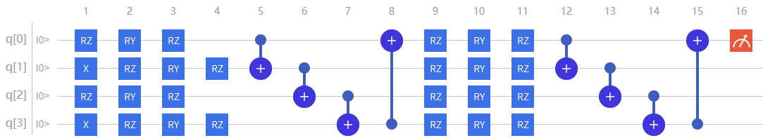
Quantum circuit
The variable component sub-circuit usually defines a sub-circuit, which is a basic circuit architecture, and complex variational circuits can be constructed by repeating layers.
Our circuit layer consists of multiple rotating quantum logic gates and CNOT quantum logic gates that entangle each qubit with its neighboring qubits.
We also need a circuit to encode classical data into a quantum state, so that the output of the circuit measurement is related to the input.
In this example, we encode the binary input onto the qubits in the corresponding order. For example, the input data 1101 is encoded into 4 qubits.
This example uses pyqpanda3.
import pyqpanda3.core as pq
from pyvqnet.nn.module import Module
from pyvqnet.optim.sgd import SGD
from pyvqnet.nn.loss import CategoricalCrossEntropy
from pyvqnet.tensor.tensor import QTensor
from pyvqnet.data import data_generator as dataloader

from pyvqnet.qnn.pq3.quantumlayer import QuantumLayer
from pyvqnet.qnn.pq3.measure import probs_measure
qnum = 4
def qvc_circuits(input,weights):

    qlist = range(qnum)
    machine =pq.CPUQVM()
    def get_cnot(nqubits):
        cir = pq.QCircuit()
        for i in range(len(nqubits)-1):
            cir << pq.CNOT(nqubits[i],nqubits[i+1])
        cir << pq.CNOT(nqubits[len(nqubits)-1],nqubits[0])
        return cir

    def build_circult(weights, xx, nqubits):

        def Rot(weights_j, qubits):
            circult = pq.QCircuit()
            circult << pq.RZ(qubits, weights_j[0])
            circult << pq.RY(qubits, weights_j[1])
            circult << pq.RZ(qubits, weights_j[2])
            return circult
        def basisstate():
            circult = pq.QCircuit()
            for i in range(len(nqubits)):
                if xx[i] == 1:
                    circult << pq.X(nqubits[i])
            return circult

        circult = pq.QCircuit()
        circult << basisstate()

        for i in range(weights.shape[0]):

            weights_i = weights[i,:,:]
            for j in range(len(nqubits)):
                weights_j = weights_i[j]
                circult << Rot(weights_j,nqubits[j])
            cnots = get_cnot(nqubits)
            circult << cnots

        circult << pq.Z(nqubits[0])

        prog = pq.QProg()
        prog << circult
        return prog

    weights = weights.reshape([2,4,3])
    prog = build_circult(weights,input,qlist)
    prob = probs_measure(machine,prog,qlist[0])

    return prob
Model building
We have defined variable quantum circuits qvc_circuits .
We hope to use it in our VQNet’s automatic differentiation framework,
to take advantage of VQNet’s optimization fucntions for model training.
We define a Model class, which inherits from the abstract class Module.
The model uses the pyvqnet.qnn.pq3.QuantumLayer class, which is a quantum computing layer that can be automatically differentiated.
qvc_circuits is the quantum circuit we want to run,
24 is the number of all quantum circuit parameters that need to be trained.
class Model(Module):
   def __init__(self):
       super(Model, self).__init__()
       self.qvc = QuantumLayer(qvc_circuits,24)

   def forward(self, x):
       return self.qvc(x)
Model training and testing
We use pre-generated random binary numbers and their odd and even labels. The data as follows.
import numpy as np
import os
qvc_train_data = [0,1,0,0,1,
0, 1, 0, 1, 0,
0, 1, 1, 0, 0,
0, 1, 1, 1, 1,
1, 0, 0, 0, 1,
1, 0, 0, 1, 0,
1, 0, 1, 0, 0,
1, 0, 1, 1, 1,
1, 1, 0, 0, 0,
1, 1, 0, 1, 1,
1, 1, 1, 0, 1,
1, 1, 1, 1, 0]
qvc_test_data= [0, 0, 0, 0, 0,
0, 0, 0, 1, 1,
0, 0, 1, 0, 1,
0, 0, 1, 1, 0]

def get_data(dataset_str):
    if dataset_str == "train":
        datasets = np.array(qvc_train_data)

    else:
        datasets = np.array(qvc_test_data)

    datasets = datasets.reshape([-1,5])
    data = datasets[:,:-1]
    label = datasets[:,-1].astype(int)
    label = np.eye(2)[label].reshape(-1,2)
    return data, label
Model forwarding, loss function calculation, reverse calculation, optimizer calculation can perform like the general neural network training mode,until the number of iterations reaches the preset value. The training data used is generated above, and the test data is qvc_test_data and train data is qvc_train_data.
def get_accuary(result,label):
    result,label = np.array(result.data), np.array(label.data)
    score = np.sum(np.argmax(result,axis=1)==np.argmax(label,1))
    return score

model = Model()

optimizer = SGD(model.parameters(),lr =0.1)

batch_size = 3

epoch = 20

loss = CategoricalCrossEntropy()

model.train()
datas,labels = get_data("train")

for i in range(epoch):
    count=0
    sum_loss = 0
    accuary = 0
    t = 0
    for data,label in dataloader(datas,labels,batch_size,False):
        optimizer.zero_grad()
        data,label = QTensor(data), QTensor(label)

        result = model(data)

        loss_b = loss(label,result)
        loss_b.backward()
        optimizer._step()
        sum_loss += loss_b.item()
        count+=batch_size
        accuary += get_accuary(result,label)
        t = t + 1

    print(f"epoch:{i}, #### loss:{sum_loss/count} #####accuray:{accuary/count}")

model.eval()
count = 0
test_data,test_label = get_data("test")
test_batch_size = 1
accuary = 0
sum_loss = 0
for testd,testl in dataloader(test_data,test_label,test_batch_size):
    testd = QTensor(testd)
    test_result = model(testd)
    test_loss = loss(testl,test_result)
    sum_loss += test_loss
    count+=test_batch_size
    accuary += get_accuary(test_result,testl)
print(f"test:--------------->loss:{sum_loss/count} #####accuray:{accuary/count}")
epoch:0, #### loss:0.20194714764753977 #####accuray:0.6666666666666666
epoch:1, #### loss:0.19724808633327484 #####accuray:0.8333333333333334
epoch:2, #### loss:0.19266503552595773 #####accuray:1.0
epoch:3, #### loss:0.18812804917494455 #####accuray:1.0
epoch:4, #### loss:0.1835678368806839 #####accuray:1.0
epoch:5, #### loss:0.1789149840672811 #####accuray:1.0
epoch:6, #### loss:0.17410411685705185 #####accuray:1.0
epoch:7, #### loss:0.16908332953850427 #####accuray:1.0
epoch:8, #### loss:0.16382796317338943 #####accuray:1.0
epoch:9, #### loss:0.15835540741682053 #####accuray:1.0
epoch:10, #### loss:0.15273457020521164 #####accuray:1.0
epoch:11, #### loss:0.14708336691061655 #####accuray:1.0
epoch:12, #### loss:0.14155150949954987 #####accuray:1.0
epoch:13, #### loss:0.1362930883963903 #####accuray:1.0
epoch:14, #### loss:0.1314386005202929 #####accuray:1.0
epoch:15, #### loss:0.12707658857107162 #####accuray:1.0
epoch:16, #### loss:0.123248390853405 #####accuray:1.0
epoch:17, #### loss:0.11995399743318558 #####accuray:1.0
epoch:18, #### loss:0.1171633576353391 #####accuray:1.0
epoch:19, #### loss:0.11482855677604675 #####accuray:1.0
[0.3412148654]
test:--------------->loss:QTensor(0.3412148654, requires_grad=True) #####accuray:1.0
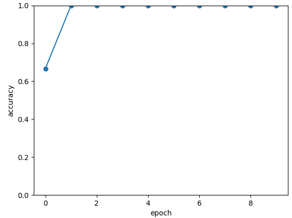
The following picture illustrates the curve of model’s accuracy:
2. data re-uploading algorithm
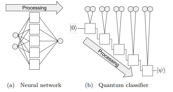
In a neural network, each neuron receives information from all neurons in the upper layer (Figure a). In contrast, the single-bit quantum classifier accepts the previous information processing unit and input (Figure b). For traditional quantum circuits, when the data is uploaded, the result can be obtained directly through several unitary transformations \(U(\theta_1,\theta_2,\theta_3)\).However, in the Quantum Data Re upLoading (QDRL) task, the data needs to be re-uploaded before every unitary transformation.
Comparison of QDRL and classic neural network schematics
import sys
sys.path.insert(0, "../")
import numpy as np
from pyvqnet.nn.linear import Linear
from pyvqnet.qnn.qdrl.vqnet_model import vmodel
from pyvqnet.optim import sgd
from pyvqnet.nn.loss import CategoricalCrossEntropy
from pyvqnet.tensor.tensor import QTensor
from pyvqnet.nn.module import Module
import matplotlib.pyplot as plt
import matplotlib
from pyvqnet.data import data_generator as get_minibatch_data
try:
    matplotlib.use("TkAgg")
except:
    print("Can not use matplot TkAgg")
    pass

np.random.seed(42)

num_layers = 3
params = np.random.uniform(size=(num_layers, 3))


class Model(Module):
    def __init__(self):

        super(Model, self).__init__()
        self.pqc = vmodel(params.shape)
        self.fc2 = Linear(2, 2)

    def forward(self, x):
        x = self.pqc(x)
        return x


def circle(samples: int, reps=np.sqrt(1 / 2)):
    data_x, data_y = [], []
    for _ in range(samples):
        x = np.random.rand(2)
        y = [0, 1]
        if np.linalg.norm(x) < reps:
            y = [1, 0]
        data_x.append(x)
        data_y.append(y)
    return np.array(data_x), np.array(data_y)


def plot_data(x, y, fig=None, ax=None):

    if fig is None:
        fig, ax = plt.subplots(1, 1, figsize=(5, 5))
    reds = y == 0
    blues = y == 1
    ax.scatter(x[reds, 0], x[reds, 1], c="red", s=20, edgecolor="k")
    ax.scatter(x[blues, 0], x[blues, 1], c="blue", s=20, edgecolor="k")
    ax.set_xlabel("$x_1$")
    ax.set_ylabel("$x_2$")


def get_score(pred, label):
    pred, label = np.array(pred.data), np.array(label.data)
    score = np.sum(np.argmax(pred, axis=1) == np.argmax(label, 1))
    return score


model = Model()
optimizer = sgd.SGD(model.parameters(), lr=1)


def train():
    """
    Main function for train qdrl model
    """
    batch_size = 5
    model.train()
    x_train, y_train = circle(500)
    x_train = np.hstack((x_train, np.ones((x_train.shape[0], 1))))  # 500*3

    epoch = 10
    print("start training...........")
    for i in range(epoch):
        accuracy = 0
        count = 0
        loss = 0
        for data, label in get_minibatch_data(x_train, y_train, batch_size):
            optimizer.zero_grad()

            data, label = QTensor(data), QTensor(label)

            output = model(data)

            loss_fun = CategoricalCrossEntropy()
            losss = loss_fun(label, output)

            losss.backward()

            optimizer._step()
            accuracy += get_score(output, label)

            loss += losss.item()

            count += batch_size

        print(f"epoch:{i}, train_accuracy_for_each_batch:{accuracy/count}")
        print(f"epoch:{i}, train_loss_for_each_batch:{loss/count}")


def test():
    batch_size = 5
    model.eval()
    print("start eval...................")
    x_test, y_test = circle(500)
    test_accuracy = 0
    count = 0
    x_test = np.hstack((x_test, np.ones((x_test.shape[0], 1))))

    for test_data, test_label in get_minibatch_data(x_test, y_test,
                                                    batch_size):

        test_data, test_label = QTensor(test_data), QTensor(test_label)
        output = model(test_data)
        test_accuracy += get_score(output, test_label)
        count += batch_size
    print(f"test_accuracy:{test_accuracy/count}")


if __name__ == "__main__":
    train()
    test()
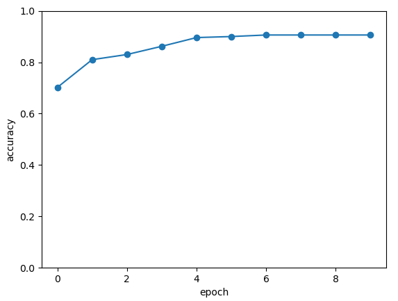
The following picture illustrates the curve of model’s accuracy:
3. VSQL: Variational Shadow Quantum Learning for Classification Model
Using variable quantum circuits to construct a two-class classification model, comparing the classification accuracy with a neural network with similar parameter accuracy, the accuracy of the two is similar. The quantity of parameters of quantum circuits is much smaller than that of classical neural networks. The algorithm is based on the paper: Variational Shadow Quantum Learning for Classification Model to reproduce.
Following figure shows the architecture of VSQL algorithm:
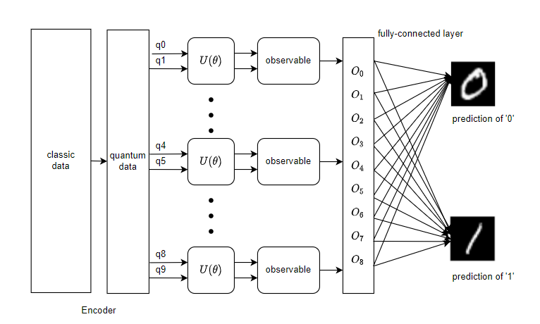
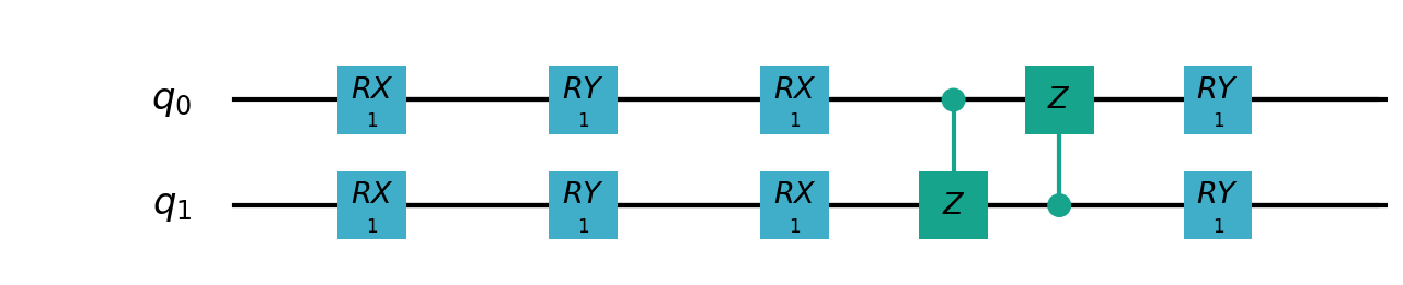
Following figures show the local quantum circuits structure on each qubits:


import sys
sys.path.insert(0, "../")
import os
import os.path
import struct
import gzip
from pyvqnet.nn.module import Module
from pyvqnet.nn.loss import CategoricalCrossEntropy
from pyvqnet.optim.adam import Adam
from pyvqnet.data.data import data_generator
from pyvqnet.tensor import tensor
from pyvqnet.qnn.measure import expval
from pyvqnet.qnn.quantumlayer import QuantumLayer
from pyvqnet.qnn.template import AmplitudeEmbeddingCircuit
from pyvqnet.nn.linear import Linear
import numpy as np
import pyqpanda as pq
import matplotlib.pyplot as plt
import matplotlib
try:
    matplotlib.use("TkAgg")
except:
    print("Can not use matplot TkAgg")
    pass

try:
    import urllib.request
except ImportError:
    raise ImportError("You should use Python 3.x")

url_base = 'https://ossci-datasets.s3.amazonaws.com/mnist/'
key_file = {
    "train_img": "train-images-idx3-ubyte.gz",
    "train_label": "train-labels-idx1-ubyte.gz",
    "test_img": "t10k-images-idx3-ubyte.gz",
    "test_label": "t10k-labels-idx1-ubyte.gz"
}


def _download(dataset_dir, file_name):
    """
    Download function for mnist dataset file
    """
    file_path = dataset_dir + "/" + file_name

    if os.path.exists(file_path):
        with gzip.GzipFile(file_path) as file:
            file_path_ungz = file_path[:-3].replace("\\", "/")
            if not os.path.exists(file_path_ungz):
                open(file_path_ungz, "wb").write(file.read())
        return

    print("Downloading " + file_name + " ... ")
    urllib.request.urlretrieve(url_base + file_name, file_path)
    if os.path.exists(file_path):
        with gzip.GzipFile(file_path) as file:
            file_path_ungz = file_path[:-3].replace("\\", "/")
            file_path_ungz = file_path_ungz.replace("-idx", ".idx")
            if not os.path.exists(file_path_ungz):
                open(file_path_ungz, "wb").write(file.read())
    print("Done")


def download_mnist(dataset_dir):
    for v in key_file.values():
        _download(dataset_dir, v)


if not os.path.exists("./result"):
    os.makedirs("./result")
else:
    pass


def circuits_of_vsql(x, weights, qlist, clist, machine):
    """
    VSQL model of quantum circuits
    """
    weights = weights.reshape([depth + 1, 3, n_qsc])

    def subcir(weights, qlist, depth, n_qsc, n_start):
        cir = pq.QCircuit()

        for i in range(n_qsc):
            cir.insert(pq.RX(qlist[n_start + i], weights[0][0][i]))
            cir.insert(pq.RY(qlist[n_start + i], weights[0][1][i]))
            cir.insert(pq.RX(qlist[n_start + i], weights[0][2][i]))
        for repeat in range(1, depth + 1):
            for i in range(n_qsc - 1):
                cir.insert(pq.CNOT(qlist[n_start + i], qlist[n_start + i + 1]))
            cir.insert(pq.CNOT(qlist[n_start + n_qsc - 1], qlist[n_start]))
            for i in range(n_qsc):
                cir.insert(pq.RY(qlist[n_start + i], weights[repeat][1][i]))

        return cir

    def get_pauli_str(n_start, n_qsc):
        pauli_str = ",".join("X" + str(i)
                            for i in range(n_start, n_start + n_qsc))
        return {pauli_str: 1.0}

    f_i = []
    origin_in = AmplitudeEmbeddingCircuit(x, qlist)
    for st in range(n - n_qsc + 1):
        psd = get_pauli_str(st, n_qsc)
        cir = pq.QCircuit()
        cir.insert(origin_in)
        cir.insert(subcir(weights, qlist, depth, n_qsc, st))
        prog = pq.QProg()
        prog.insert(cir)

        f_ij = expval(machine, prog, psd, qlist)
        f_i.append(f_ij)
    f_i = np.array(f_i)
    return f_i


#GLOBAL VAR
n = 10
n_qsc = 2
depth = 1


class QModel(Module):
    """
    Model of VSQL
    """
    def __init__(self):
        super().__init__()
        self.vq = QuantumLayer(circuits_of_vsql, (depth + 1) * 3 * n_qsc,
                            "cpu", 10)
        self.fc = Linear(n - n_qsc + 1, 2)

    def forward(self, x):
        x = self.vq(x)
        x = self.fc(x)

        return x


class Model(Module):
    def __init__(self):
        super().__init__()
        self.fc1 = Linear(input_channels=28 * 28, output_channels=2)

    def forward(self, x):

        x = tensor.flatten(x, 1)
        x = self.fc1(x)
        return x


def load_mnist(dataset="training_data", digits=np.arange(2), path="./"):
    """
    load mnist data
    """
    from array import array as pyarray
    download_mnist(path)
    if dataset == "training_data":
        fname_image = os.path.join(path, "train-images.idx3-ubyte").replace(
            "\\", "/")
        fname_label = os.path.join(path, "train-labels.idx1-ubyte").replace(
            "\\", "/")
    elif dataset == "testing_data":
        fname_image = os.path.join(path, "t10k-images.idx3-ubyte").replace(
            "\\", "/")
        fname_label = os.path.join(path, "t10k-labels.idx1-ubyte").replace(
            "\\", "/")
    else:
        raise ValueError("dataset must be 'training_data' or 'testing_data'")

    flbl = open(fname_label, "rb")
    _, size = struct.unpack(">II", flbl.read(8))

    lbl = pyarray("b", flbl.read())
    flbl.close()

    fimg = open(fname_image, "rb")
    _, size, rows, cols = struct.unpack(">IIII", fimg.read(16))
    img = pyarray("B", fimg.read())
    fimg.close()

    ind = [k for k in range(size) if lbl[k] in digits]
    num = len(ind)
    images = np.zeros((num, rows, cols), dtype=np.float32)

    labels = np.zeros((num, 1), dtype=int)
    for i in range(len(ind)):
        images[i] = np.array(img[ind[i] * rows * cols:(ind[i] + 1) * rows *
                                cols]).reshape((rows, cols))
        labels[i] = lbl[ind[i]]

    return images, labels


def run_vsql():
    """
    VQSL MODEL
    """
    digits = [0, 1]
    x_train, y_train = load_mnist("training_data", digits)
    x_train = x_train / 255
    y_train = y_train.reshape(-1, 1)
    y_train = np.eye(len(digits))[y_train].reshape(-1, len(digits)).astype(
        np.int64)
    x_test, y_test = load_mnist("testing_data", digits)
    x_test = x_test / 255
    y_test = y_test.reshape(-1, 1)
    y_test = np.eye(len(digits))[y_test].reshape(-1,
                                                len(digits)).astype(np.int64)

    x_train_list = []
    x_test_list = []
    for i in range(x_train.shape[0]):
        x_train_list.append(
            np.pad(x_train[i, :, :].flatten(), (0, 240),
                constant_values=(0, 0)))
    x_train = np.array(x_train_list)

    for i in range(x_test.shape[0]):
        x_test_list.append(
            np.pad(x_test[i, :, :].flatten(), (0, 240),
                constant_values=(0, 0)))

    x_test = np.array(x_test_list)

    x_train = x_train[:500]
    y_train = y_train[:500]

    x_test = x_test[:100]
    y_test = y_test[:100]
    print("model start")
    model = QModel()

    optimizer = Adam(model.parameters(), lr=0.1)

    model.train()
    result_file = open("./result/vqslrlt.txt", "w")
    for epoch in range(1, 3):

        model.train()
        full_loss = 0
        n_loss = 0
        n_eval = 0
        batch_size = 1
        correct = 0
        for x, y in data_generator(x_train,
                                y_train,
                                batch_size=batch_size,
                                shuffle=True):
            optimizer.zero_grad()
            try:
                x = x.reshape(batch_size, 1024)
            except:
                x = x.reshape(-1, 1024)

            output = model(x)
            cceloss = CategoricalCrossEntropy()
            loss = cceloss(y, output)
            loss.backward()
            optimizer._step()

            full_loss += loss.item()
            n_loss += batch_size
            np_output = np.array(output.data, copy=False)
            mask = np_output.argmax(1) == y.argmax(1)
            correct += sum(mask)
            print(f" n_loss {n_loss} Train Accuracy: {correct/n_loss} ")
        print(f"Train Accuracy: {correct/n_loss} ")
        print(f"Epoch: {epoch}, Loss: {full_loss / n_loss}")
        result_file.write(f"{epoch}\t{full_loss / n_loss}\t{correct/n_loss}\t")

        # Evaluation
        model.eval()
        print("eval")
        correct = 0
        full_loss = 0
        n_loss = 0
        n_eval = 0
        batch_size = 1
        for x, y in data_generator(x_test,
                                y_test,
                                batch_size=batch_size,
                                shuffle=True):
            x = x.reshape(1, 1024)
            output = model(x)

            cceloss = CategoricalCrossEntropy()
            loss = cceloss(y, output)
            full_loss += loss.item()

            np_output = np.array(output.data, copy=False)
            mask = np_output.argmax(1) == y.argmax(1)
            correct += sum(mask)
            n_eval += 1
            n_loss += 1

        print(f"Eval Accuracy: {correct/n_eval}")
        result_file.write(f"{full_loss / n_loss}\t{correct/n_eval}\n")

    result_file.close()
    del model
    print("\ndone vqsl\n")


if __name__ == "__main__":

    run_vsql()
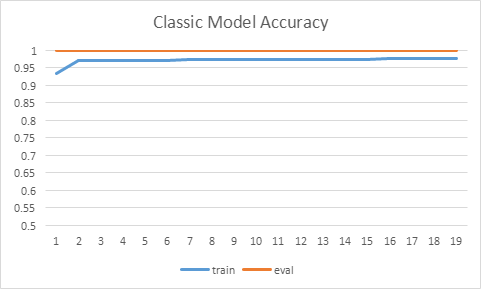
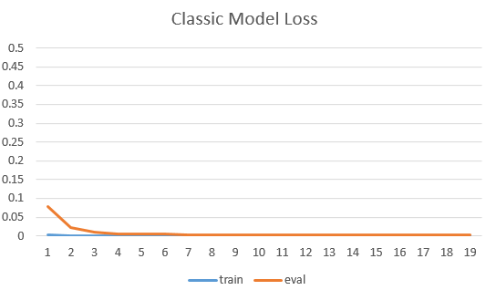
The following shows the curve of model’s accuracy and loss:
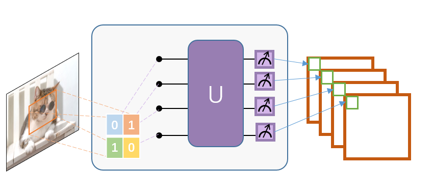
4.Quanvolution for image classification
In this example, we implement a Quantum Convolutional Neural Network, a type originally introduced in the paper Quanvolutional Neural Networks: Powering Image Recognition with Quantum Circuits method.
Similar to classic convolution, Quanvolution has the following steps:
A small region of the input image, in our case a 2×2 square of classical data, is embedded into the quantum circuit.
In this example, this is achieved by applying parameterized rotating logic gates to qubits initialized in the ground state. The convolutional kernel here generates variational circuits from stochastic circuits proposed in ref.
Finally, the quantum system is measured to obtain a list of classical expected values.
Similar to a classic convolutional layer, each expected value is mapped to a different channel of a single output pixel.
Repeating the same process over different regions, the complete input image can be scanned, producing an output object that will be constructed as a multi-channel image.
In order to perform classification tasks, this example uses the classic fully connected layer Linear to perform classification tasks after Quanvolution obtains the measurement values.
The main difference from classical convolution is that Quanvolution can generate highly complex kernels whose computation is at least in principle classically intractable.
Mnist dataset definition
import os
import os.path
import struct
import gzip
import sys
sys.path.insert(0, "../")
from pyvqnet.nn.module import Module
from pyvqnet.nn.loss import NLL_Loss
from pyvqnet.optim.adam import Adam
from pyvqnet.data.data import data_generator
from pyvqnet.tensor import tensor
from pyvqnet.qnn.measure import expval
from pyvqnet.nn.linear import Linear
import numpy as np
from pyvqnet.qnn.qcnn import Quanvolution
import matplotlib.pyplot as plt
import matplotlib
try:
    matplotlib.use("TkAgg")
except:
    print("Can not use matplot TkAgg")
    pass

try:
    import urllib.request
except ImportError:
    raise ImportError("You should use Python 3.x")

url_base = 'https://ossci-datasets.s3.amazonaws.com/mnist/'
key_file = {
    "train_img": "train-images-idx3-ubyte.gz",
    "train_label": "train-labels-idx1-ubyte.gz",
    "test_img": "t10k-images-idx3-ubyte.gz",
    "test_label": "t10k-labels-idx1-ubyte.gz"
}


def _download(dataset_dir, file_name):
    """
    Download function for mnist dataset file
    """
    file_path = dataset_dir + "/" + file_name

    if os.path.exists(file_path):
        with gzip.GzipFile(file_path) as file:
            file_path_ungz = file_path[:-3].replace("\\", "/")
            if not os.path.exists(file_path_ungz):
                open(file_path_ungz, "wb").write(file.read())
        return

    print("Downloading " + file_name + " ... ")
    urllib.request.urlretrieve(url_base + file_name, file_path)
    if os.path.exists(file_path):
        with gzip.GzipFile(file_path) as file:
            file_path_ungz = file_path[:-3].replace("\\", "/")
            file_path_ungz = file_path_ungz.replace("-idx", ".idx")
            if not os.path.exists(file_path_ungz):
                open(file_path_ungz, "wb").write(file.read())
    print("Done")


def download_mnist(dataset_dir):
    for v in key_file.values():
        _download(dataset_dir, v)


if not os.path.exists("./result"):
    os.makedirs("./result")
else:
    pass


def load_mnist(dataset="training_data", digits=np.arange(10), path="./"):
    """
    load mnist data
    """
    from array import array as pyarray
    download_mnist(path)
    if dataset == "training_data":
        fname_image = os.path.join(path, "train-images.idx3-ubyte").replace(
            "\\", "/")
        fname_label = os.path.join(path, "train-labels.idx1-ubyte").replace(
            "\\", "/")
    elif dataset == "testing_data":
        fname_image = os.path.join(path, "t10k-images.idx3-ubyte").replace(
            "\\", "/")
        fname_label = os.path.join(path, "t10k-labels.idx1-ubyte").replace(
            "\\", "/")
    else:
        raise ValueError("dataset must be 'training_data' or 'testing_data'")

    flbl = open(fname_label, "rb")
    _, size = struct.unpack(">II", flbl.read(8))

    lbl = pyarray("b", flbl.read())
    flbl.close()

    fimg = open(fname_image, "rb")
    _, size, rows, cols = struct.unpack(">IIII", fimg.read(16))
    img = pyarray("B", fimg.read())
    fimg.close()

    ind = [k for k in range(size) if lbl[k] in digits]
    num = len(ind)
    images = np.zeros((num, rows, cols))

    labels = np.zeros((num, 1), dtype=int)
    for i in range(len(ind)):
        images[i] = np.array(img[ind[i] * rows * cols:(ind[i] + 1) * rows *
                                cols]).reshape((rows, cols))
        labels[i] = lbl[ind[i]]

    return images, labels
Module definition and process function’s definition
class QModel(Module):

    def __init__(self):
        super().__init__()
        self.vq = Quanvolution([4, 2], (2, 2))
        self.fc = Linear(4 * 14 * 14, 10)

    def forward(self, x):
        x = self.vq(x)
        x = tensor.flatten(x, 1)
        x = self.fc(x)
        x = tensor.log_softmax(x)
        return x


def run_quanvolution():

    digit = 10
    x_train, y_train = load_mnist("training_data", digits=np.arange(digit))
    x_train = x_train / 255

    y_train = y_train.flatten()

    x_test, y_test = load_mnist("testing_data", digits=np.arange(digit))

    x_test = x_test / 255
    y_test = y_test.flatten()

    x_train = x_train[:500]
    y_train = y_train[:500]

    x_test = x_test[:100]
    y_test = y_test[:100]

    print("model start")
    model = QModel()

    optimizer = Adam(model.parameters(), lr=5e-3)

    model.train()
    result_file = open("quanvolution.txt", "w")

    cceloss = NLL_Loss()
    N_EPOCH = 15

    for epoch in range(1, N_EPOCH):

        model.train()
        full_loss = 0
        n_loss = 0
        n_eval = 0
        batch_size = 10
        correct = 0
        for x, y in data_generator(x_train,
                                y_train,
                                batch_size=batch_size,
                                shuffle=True):
            optimizer.zero_grad()
            try:
                x = x.reshape(batch_size, 1, 28, 28)
            except:
                x = x.reshape(-1, 1, 28, 28)

            output = model(x)

            loss = cceloss(y, output)
            print(f"loss {loss}")
            loss.backward()
            optimizer._step()

            full_loss += loss.item()
            n_loss += batch_size
            np_output = np.array(output.data, copy=False)
            mask = np_output.argmax(1) == y

            correct += sum(mask)
            print(f"correct {correct}")
        print(f"Train Accuracy: {correct/n_loss}%")
        print(f"Epoch: {epoch}, Loss: {full_loss / n_loss}")
        result_file.write(f"{epoch}\t{full_loss / n_loss}\t{correct/n_loss}\t")

        # Evaluation
        model.eval()
        print("eval")
        correct = 0
        full_loss = 0
        n_loss = 0
        n_eval = 0
        batch_size = 1
        for x, y in data_generator(x_test,
                                y_test,
                                batch_size=batch_size,
                                shuffle=True):
            x = x.reshape(-1, 1, 28, 28)
            output = model(x)

            loss = cceloss(y, output)
            full_loss += loss.item()

            np_output = np.array(output.data, copy=False)
            mask = np_output.argmax(1) == y
            correct += sum(mask)
            n_eval += 1
            n_loss += 1

        print(f"Eval Accuracy: {correct/n_eval}")
        result_file.write(f"{full_loss / n_loss}\t{correct/n_eval}\n")

    result_file.close()
    del model
    print("\ndone\n")


if __name__ == "__main__":

    run_quanvolution()
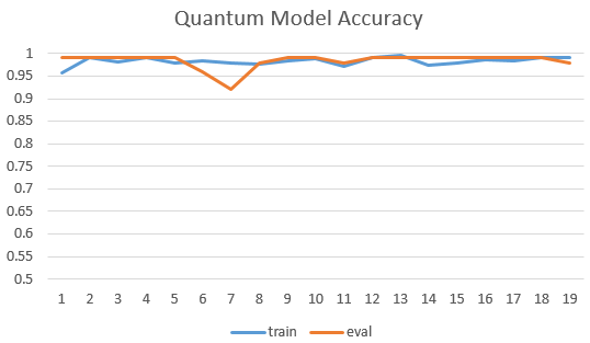
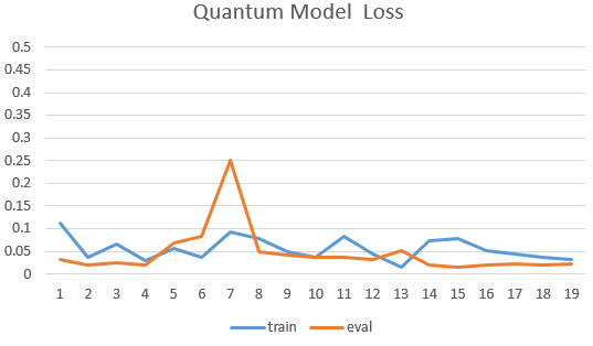
Training set, verification set loss, training set, verification set classification accuracy with Epoch transformation.
# epoch train_loss      train_accuracy eval_loss    eval_accuracy
# 1 0.2488900272846222      0.232   1.7297331787645818      0.39
# 2 0.12281704187393189     0.646   1.201728610806167       0.61
# 3 0.08001763761043548     0.772   0.8947569639235735      0.73
# 4 0.06211201059818268     0.83    0.777864265316166       0.74
# 5 0.052190632969141004    0.858   0.7291000287979841      0.76
# 6 0.04542196464538574     0.87    0.6764470228599384      0.8
# 7 0.04029472427070141     0.896   0.6153804161818698      0.79
# 8 0.03600500610470772     0.902   0.5644993982824963      0.81
# 9 0.03230033944547176     0.916   0.528938240573043       0.81
# 10        0.02912954458594322     0.93    0.5058713140769396      0.83
# 11        0.026443827204406262    0.936   0.49064547760412097     0.83
# 12        0.024144304402172564    0.942   0.4800815625616815      0.82
# 13        0.022141477409750223    0.952   0.4724775951183983      0.83
# 14        0.020372112181037665    0.956   0.46692863543197743     0.83
Quantum AutoEncoder Demo
1.Quantum AutoEncoder
The classic autoencoder is a neural network that can learn high-efficiency low-dimensional representations of data in a high-dimensional space. The task of the autoencoder is to map x to a low-dimensional point y given an input x, so that x can be recovered from y. The structure of the underlying autoencoder network can be selected to represent the data in a smaller dimension, thereby effectively compressing the input. Inspired by this idea, the model of quantum autoencoder is used to perform similar tasks on quantum data. Quantum autoencoders are trained to compress specific data sets of quantum states, and classical compression algorithms cannot be used. The parameters of the quantum autoencoder are trained using classical optimization algorithms. We show an example of a simple programmable circuit, which can be trained as an efficient autoencoder. We apply our model in the context of quantum simulation to compress the Hubbard model and the ground state of the Hamiltonian. This algorithm is based on Quantum autoencoders for efficient compression of quantum data .
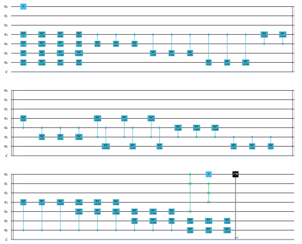
QAE quantum circuits:
import os
import sys
sys.path.insert(0,'../')
import numpy as np
from pyvqnet.nn.module import Module
from pyvqnet.nn.loss import fidelityLoss
from pyvqnet.optim.adam import Adam
from pyvqnet.data.data import data_generator
from pyvqnet.qnn.qae.qae import QAElayer
import matplotlib.pyplot as plt
import matplotlib
try:
matplotlib.use('TkAgg')
except:
pass
try:
import urllib.request
except ImportError:
raise ImportError('You should use Python 3.x')
import os.path
import gzip
url_base = 'https://ossci-datasets.s3.amazonaws.com/mnist/'
key_file = {
'train_img':'train-images-idx3-ubyte.gz',
'train_label':'train-labels-idx1-ubyte.gz',
'test_img':'t10k-images-idx3-ubyte.gz',
'test_label':'t10k-labels-idx1-ubyte.gz'
}
def _download(dataset_dir,file_name):
file_path = dataset_dir + "/" + file_name
if os.path.exists(file_path):
with gzip.GzipFile(file_path) as f:
file_path_ungz = file_path[:-3].replace('\\', '/')
if not os.path.exists(file_path_ungz):
open(file_path_ungz,"wb").write(f.read())
return
print("Downloading " + file_name + " ... ")
urllib.request.urlretrieve(url_base + file_name, file_path)
if os.path.exists(file_path):
with gzip.GzipFile(file_path) as f:
file_path_ungz = file_path[:-3].replace('\\', '/')
file_path_ungz = file_path_ungz.replace('-idx', '.idx')
if not os.path.exists(file_path_ungz):
open(file_path_ungz,"wb").write(f.read())
print("Done")
def download_mnist(dataset_dir):
for v in key_file.values():
_download(dataset_dir,v)
class Model(Module):
def __init__(self, trash_num: int = 2, total_num: int = 7):
super().__init__()
self.pqc = QAElayer(trash_num, total_num)
def forward(self, x):
x = self.pqc(x)
return x
def load_mnist(dataset="training_data", digits=np.arange(2), path="./"):
import os, struct
from array import array as pyarray
download_mnist(path)
if dataset == "training_data":
fname_image = os.path.join(path, 'train-images.idx3-ubyte').replace('\\', '/')
fname_label = os.path.join(path, 'train-labels.idx1-ubyte').replace('\\', '/')
elif dataset == "testing_data":
fname_image = os.path.join(path, 't10k-images.idx3-ubyte').replace('\\', '/')
fname_label = os.path.join(path, 't10k-labels.idx1-ubyte').replace('\\', '/')
else:
raise ValueError("dataset must be 'training_data' or 'testing_data'")
flbl = open(fname_label, 'rb')
magic_nr, size = struct.unpack(">II", flbl.read(8))
lbl = pyarray("b", flbl.read())
flbl.close()
fimg = open(fname_image, 'rb')
magic_nr, size, rows, cols = struct.unpack(">IIII", fimg.read(16))
img = pyarray("B", fimg.read())
fimg.close()
ind = [k for k in range(size) if lbl[k] in digits]
N = len(ind)
images = np.zeros((N, rows, cols))
labels = np.zeros((N, 1), dtype=int)
for i in range(len(ind)):
images[i] = np.array(img[ind[i] * rows * cols: (ind[i] + 1) * rows * cols]).reshape((rows, cols))
labels[i] = lbl[ind[i]]
return images, labels
def run2():
##load dataset
x_train, y_train = load_mnist("training_data")
x_train = x_train / 255
x_test, y_test = load_mnist("testing_data")
x_test = x_test / 255
x_train = x_train.reshape([-1, 1, 28, 28])
x_test = x_test.reshape([-1, 1, 28, 28])
x_train = x_train[:100, :, :, :]
x_train = np.resize(x_train, [x_train.shape[0], 1, 2, 2])
x_test = x_test[:10, :, :, :]
x_test = np.resize(x_test, [x_test.shape[0], 1, 2, 2])
encode_qubits = 4
latent_qubits = 2
trash_qubits = encode_qubits - latent_qubits
total_qubits = 1 + trash_qubits + encode_qubits
print("model start")
model = Model(trash_qubits, total_qubits)
optimizer = Adam(model.parameters(), lr=0.005)
model.train()
F1 = open("rlt.txt", "w")
loss_list = []
loss_list_test = []
fidelity_train = []
fidelity_val = []
for epoch in range(1, 10):
running_fidelity_train = 0
running_fidelity_val = 0
print(f"epoch {epoch}")
model.train()
full_loss = 0
n_loss = 0
n_eval = 0
batch_size = 1
correct = 0
iter = 0
if epoch %5 ==1:
optimizer.lr = optimizer.lr *0.5
for x, y in data_generator(x_train, y_train, batch_size=batch_size, shuffle=True): #shuffle batch rather than data
x = x.reshape((-1, encode_qubits))
x = np.concatenate((np.zeros([batch_size, 1 + trash_qubits]), x), 1)
optimizer.zero_grad()
output = model(x)
iter += 1
np_out = np.array(output.data)
floss = fidelityLoss()
loss = floss(output)
loss_data = np.array(loss.data)
loss.backward()
running_fidelity_train += np_out[0]
optimizer._step()
full_loss += loss_data[0]
n_loss += batch_size
np_output = np.array(output.data, copy=False)
mask = np_output.argmax(1) == y.argmax(1)
correct += sum(mask)
loss_output = full_loss / n_loss
print(f"Epoch: {epoch}, Loss: {loss_output}")
loss_list.append(loss_output)
# Evaluation
model.eval()
correct = 0
full_loss = 0
n_loss = 0
n_eval = 0
batch_size = 1
for x, y in data_generator(x_test, y_test, batch_size=batch_size, shuffle=True):
x = x.reshape((-1, encode_qubits))
x = np.concatenate((np.zeros([batch_size, 1 + trash_qubits]),x),1)
output = model(x)
floss = fidelityLoss()
loss = floss(output)
loss_data = np.array(loss.data)
full_loss += loss_data[0]
running_fidelity_val += np.array(output.data)[0]
n_eval += 1
n_loss += 1
loss_output = full_loss / n_loss
print(f"Epoch: {epoch}, Loss: {loss_output}")
loss_list_test.append(loss_output)
fidelity_train.append(running_fidelity_train / 64)
fidelity_val.append(running_fidelity_val / 64)
figure_path = os.path.join(os.getcwd(), 'QAE-rate1.png')
plt.plot(loss_list, color="blue", label="train")
plt.plot(loss_list_test, color="red", label="validation")
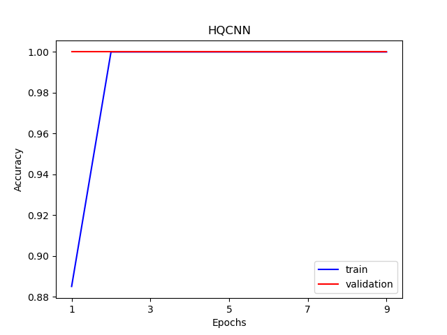
plt.title('QAE')
plt.xlabel("Epochs")
plt.ylabel("Loss")
plt.legend(loc="upper right")
plt.savefig(figure_path)
plt.show()
F1.write(f"done\n")
F1.close()
del model
if __name__ == '__main__':
run2()
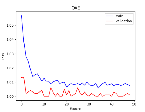
The QAE error value obtained by running the above code, the loss is 1/fidelity, tending to 1 means the fidelity is close to 1.
Quantum Circuits Structure Learning Demo
1.Quantum circuits structure learning
In the quantum circuit structure, the most frequently used quantum gates with parameters are RZ , RY , and RX gates, but which gate to use under what circumstances is a question worth studying. One method is random selection, but in this case It is very likely that the best results will not be achieved. The core goal of Quantum circuit structure learning task is to find the optimal combination of quantum gates with parameters. The approach here is that this set of optimal quantum logic gates should make the loss function to be the minimum.
"""
Quantum Circuits Strcture Learning Demo

"""
import sys
sys.path.insert(0,"../")

import copy
import pyqpanda as pq
from pyvqnet.tensor.tensor import QTensor
from pyvqnet.qnn.measure import expval
import numpy as np
import matplotlib.pyplot as plt
import matplotlib
try:
    matplotlib.use("TkAgg")
except:
    print("Can not use matplot TkAgg")
    pass

machine = pq.CPUQVM()
machine.init_qvm()
nqbits = machine.qAlloc_many(2)

def gen(param, generators, qbits, circuit):
    if generators == "X":
        circuit.insert(pq.RX(qbits, param))
    elif generators == "Y":
        circuit.insert(pq.RY(qbits, param))
    else:
        circuit.insert(pq.RZ(qbits, param))

def circuits(params, generators, circuit):
    gen(params[0], generators[0], nqbits[0], circuit)
    gen(params[1], generators[1], nqbits[1], circuit)
    circuit.insert(pq.CNOT(nqbits[0], nqbits[1]))
    prog = pq.QProg()
    prog.insert(circuit)
    return prog

def ansatz1(params: QTensor, generators):
    circuit = pq.QCircuit()
    params = params.to_numpy()
    prog = circuits(params, generators, circuit)
    return expval(machine, prog, {"Z0": 1},
                nqbits), expval(machine, prog, {"Y1": 1}, nqbits)


def ansatz2(params: QTensor, generators):
    circuit = pq.QCircuit()
    params = params.to_numpy()
    prog = circuits(params, generators, circuit)
    return expval(machine, prog, {"X0": 1}, nqbits)


def loss(params, generators):
    z, y = ansatz1(params, generators)
    x = ansatz2(params, generators)
    return 0.5 * y + 0.8 * z - 0.2 * x


def rotosolve(d, params, generators, cost, M_0):
    """
    rotosolve algorithm implementation
    """
    params[d] = np.pi / 2.0
    m0_plus = cost(QTensor(params), generators)
    params[d] = -np.pi / 2.0
    m0_minus = cost(QTensor(params), generators)
    a = np.arctan2(2.0 * M_0 - m0_plus - m0_minus,
                m0_plus - m0_minus)  # returns value in (-pi,pi]
    params[d] = -np.pi / 2.0 - a
    if params[d] <= -np.pi:
        params[d] += 2 * np.pi
    return cost(QTensor(params), generators)


def optimal_theta_and_gen_helper(index, params, generators):
    """
    find optimal varaibles
    """
    params[index] = 0.
    m0 = loss(QTensor(params), generators)  #init value
    for kind in ["X", "Y", "Z"]:
        generators[index] = kind
        params_cost = rotosolve(index, params, generators, loss, m0)
        if kind == "X" or params_cost <= params_opt_cost:
            params_opt_d = params[index]
            params_opt_cost = params_cost
            generators_opt_d = kind
    return params_opt_d, generators_opt_d


def rotoselect_cycle(params: np, generators):
    for index in range(params.shape[0]):
        params[index], generators[index] = optimal_theta_and_gen_helper(
            index, params, generators)
    return params, generators


params = QTensor(np.array([0.3, 0.25]))
params = params.to_numpy()
generator = ["X", "Y"]
generators = copy.deepcopy(generator)
epoch = 20
state_save = []
for i in range(epoch):
    state_save.append(loss(QTensor(params), generators))
    params, generators = rotoselect_cycle(params, generators)

print("Optimal generators are: {}".format(generators))
print("Optimal params are: {}".format(params))
steps = np.arange(0, epoch)


plt.plot(steps, state_save, "o-")
plt.title("rotoselect")
plt.xlabel("cycles")
plt.ylabel("cost")
plt.yticks(np.arange(-1.25, 0.80, 0.25))
plt.tight_layout()
plt.show()
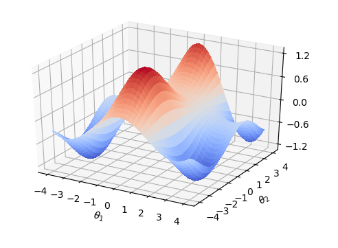
The quantum circuit structure obtained by running the above code contains \(RX\), one \(RY\)
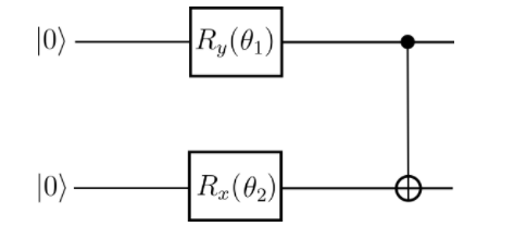
And with the parameters in the quantum gate \(\theta_1\), \(\theta_2\) change,Loss function has different values.
Hybird Quantum Classic Nerual Network Demo
1.Hybrid Quantum Classic Neural Network Model
Machine learning (ML) has become a successful interdisciplinary field that aims to extract generalizable information from data mathematically. Quantum machine learning seeks to use the principles of quantum mechanics to enhance machine learning, and vice versa. Whether your goal is to enhance classical ML algorithms by outsourcing difficult calculations to quantum computers, or use classical ML architectures to optimize quantum algorithms-both fall into the category of quantum machine learning (QML). In this chapter, we will explore how to partially quantify classical neural networks to create hybrid quantum classical neural networks. Quantum circuits are composed of quantum logic gates, and the quantum calculations implemented by these logic gates are proved to be differentiable by the paper Quantum Circuit Learning. Therefore, researchers try to put quantum circuits and classical neural network modules together for training on hybrid quantum classical machine learning tasks. We will write a simple example to implement a neural network model training task using VQNet. The purpose of this example is to demonstrate the simplicity of VQNet and encourage ML practitioners to explore the possibilities of quantum computing.
Data Preparation
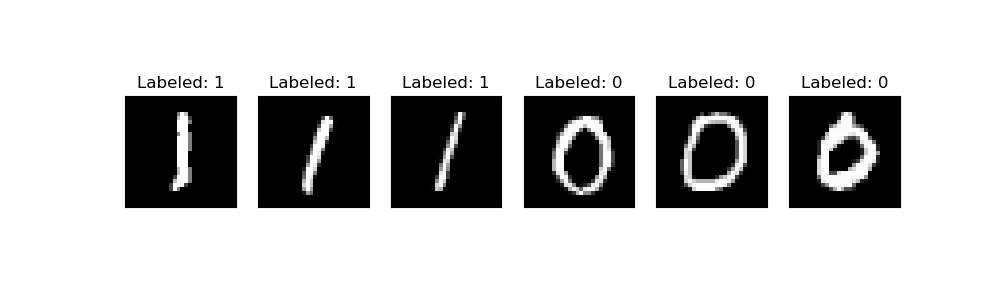
We will use MNIST datasets, the most basic neural network handwritten digit database as the classification data. We first load MNIST and filter data samples containing 0 and 1. These samples are divided into training data training_data and testing data testing_data, each of which has a dimension of 1*784.
import time
import os
import struct
import gzip
from pyvqnet.nn.module import Module
from pyvqnet.nn.linear import Linear
from pyvqnet.nn.conv import Conv2D

from pyvqnet.nn import activation as F
from pyvqnet.nn.pooling import MaxPool2D
from pyvqnet.nn.loss import CategoricalCrossEntropy
from pyvqnet.optim.adam import Adam
from pyvqnet.data.data import data_generator
from pyvqnet.tensor import tensor
from pyvqnet.tensor import QTensor
import pyqpanda as pq

import numpy as np
import matplotlib.pyplot as plt
import matplotlib
try:
    matplotlib.use("TkAgg")
except:
    print("Can not use matplot TkAgg")
    pass

try:
    import urllib.request
except ImportError:
    raise ImportError("You should use Python 3.x")

url_base = 'https://ossci-datasets.s3.amazonaws.com/mnist/'
key_file = {
    'train_img':'train-images-idx3-ubyte.gz',
    'train_label':'train-labels-idx1-ubyte.gz',
    'test_img':'t10k-images-idx3-ubyte.gz',
    'test_label':'t10k-labels-idx1-ubyte.gz'
}

def _download(dataset_dir,file_name):
    file_path = dataset_dir + "/" + file_name

    if os.path.exists(file_path):
        with gzip.GzipFile(file_path) as f:
            file_path_ungz = file_path[:-3].replace('\\', '/')
            if not os.path.exists(file_path_ungz):
                open(file_path_ungz,"wb").write(f.read())
        return

    print("Downloading " + file_name + " ... ")
    urllib.request.urlretrieve(url_base + file_name, file_path)
    if os.path.exists(file_path):
            with gzip.GzipFile(file_path) as f:
                file_path_ungz = file_path[:-3].replace('\\', '/')
                file_path_ungz = file_path_ungz.replace('-idx', '.idx')
                if not os.path.exists(file_path_ungz):
                    open(file_path_ungz,"wb").write(f.read())
    print("Done")

def download_mnist(dataset_dir):
    for v in key_file.values():
        _download(dataset_dir,v)

def load_mnist(dataset="training_data", digits=np.arange(2), path="./"):
    import os, struct
    from array import array as pyarray
    download_mnist(path)
    if dataset == "training_data":
        fname_image = os.path.join(path, 'train-images.idx3-ubyte').replace('\\', '/')
        fname_label = os.path.join(path, 'train-labels.idx1-ubyte').replace('\\', '/')
    elif dataset == "testing_data":
        fname_image = os.path.join(path, 't10k-images.idx3-ubyte').replace('\\', '/')
        fname_label = os.path.join(path, 't10k-labels.idx1-ubyte').replace('\\', '/')
    else:
        raise ValueError("dataset must be 'training_data' or 'testing_data'")

    flbl = open(fname_label, 'rb')
    magic_nr, size = struct.unpack(">II", flbl.read(8))
    lbl = pyarray("b", flbl.read())
    flbl.close()

    fimg = open(fname_image, 'rb')
    magic_nr, size, rows, cols = struct.unpack(">IIII", fimg.read(16))
    img = pyarray("B", fimg.read())
    fimg.close()

    ind = [k for k in range(size) if lbl[k] in digits]
    N = len(ind)
    images = np.zeros((N, rows, cols))
    labels = np.zeros((N, 1), dtype=int)
    for i in range(len(ind)):
        images[i] = np.array(img[ind[i] * rows * cols: (ind[i] + 1) * rows * cols]).reshape((rows, cols))
        labels[i] = lbl[ind[i]]

    return images, labels

def data_select(train_num, test_num):
    x_train, y_train = load_mnist("training_data")
    x_test, y_test = load_mnist("testing_data")
    # Train Leaving only labels 0 and 1
    idx_train = np.append(np.where(y_train == 0)[0][:train_num],
                    np.where(y_train == 1)[0][:train_num])
    x_train = x_train[idx_train]
    y_train = y_train[idx_train]
    x_train = x_train / 255
    y_train = np.eye(2)[y_train].reshape(-1, 2)
    # Test Leaving only labels 0 and 1
    idx_test = np.append(np.where(y_test == 0)[0][:test_num],
                    np.where(y_test == 1)[0][:test_num])
    x_test = x_test[idx_test]
    y_test = y_test[idx_test]
    x_test = x_test / 255
    y_test = np.eye(2)[y_test].reshape(-1, 2)
    return x_train, y_train, x_test, y_test

n_samples_show = 6

x_train, y_train, x_test, y_test = data_select(100, 50)
fig, axes = plt.subplots(nrows=1, ncols=n_samples_show, figsize=(10, 3))

for img ,targets in zip(x_test,y_test):
    if n_samples_show <= 3:
        break

    if targets[0] == 1:
        axes[n_samples_show - 1].set_title("Labeled: 0")
        axes[n_samples_show - 1].imshow(img.squeeze(), cmap='gray')
        axes[n_samples_show - 1].set_xticks([])
        axes[n_samples_show - 1].set_yticks([])
        n_samples_show -= 1

for img ,targets in zip(x_test,y_test):
    if n_samples_show <= 0:
        break

    if targets[0] == 0:
        axes[n_samples_show - 1].set_title("Labeled: 1")
        axes[n_samples_show - 1].imshow(img.squeeze(), cmap='gray')
        axes[n_samples_show - 1].set_xticks([])
        axes[n_samples_show - 1].set_yticks([])
        n_samples_show -= 1

plt.show()
Construct Quantum Circuits
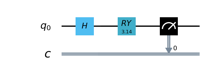
In this example, we use the pyQPanda2 , A simple quantum circuit of 1 qubit is defined. The circuit takes the output of the classical neural network layer as input,encodes quantum data through H , RY quantum logic gates, and calculates the expected value of Hamiltonian in the z direction as output.
from pyqpanda import *
import pyqpanda as pq
import numpy as np
def circuit(weights):
    num_qubits = 1
    #Use pyQPanda2 to create a simulator
    machine = pq.CPUQVM()
    machine.init_qvm()
    #Use pyQPanda2 to alloc qubits
    qubits = machine.qAlloc_many(num_qubits)
    #Use pyQPanda2 to alloc classic bits
    cbits = machine.cAlloc_many(num_qubits)
    #Construct circuits
    circuit = pq.QCircuit()
    circuit.insert(pq.H(qubits[0]))
    circuit.insert(pq.RY(qubits[0], weights[0]))
    #Construct quantum program
    prog = pq.QProg()
    prog.insert(circuit)
    #Defines measurement
    prog << measure_all(qubits, cbits)

    #run quantum with quantum measurements
    result = machine.run_with_configuration(prog, cbits, 100)

    counts = np.array(list(result.values()))
    states = np.array(list(result.keys())).astype(float)
    probabilities = counts / 100
    expectation = np.sum(states * probabilities)
    return expectation
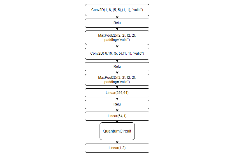
Create Hybird Model
Since quantum circuits can perform automatic differentiation calculations together with classical neural networks,
Therefore, we can use VQNet’s convolutional layer Conv2D , pooling layer MaxPool2D , fully connected layer Linear and
the quantum circuit to build model just now.
The definition of the Net and Hybrid classes inherit from the VQNet automatic differentiation module Module
and the definition of the forward calculation is defined in forward function forward(),
An automatic differentiation Model of convolution, quantum encoding, and measurement of the MNIST data is constructed to obtain the final features required for the classification task.
#Quantum computing layer front pass and the definition of gradient calculation function, which need to be inherited from the abstract class Module
from pyvqnet.native.backprop_utils import AutoGradNode
class Hybrid(Module):
    """ Hybrid quantum - Quantum layer definition """
    def __init__(self, shift):
        super(Hybrid, self).__init__()
        self.shift = shift
    def forward(self, input):
        self.input = input
        expectation_z = circuit(np.array(input.data))
        result = [[expectation_z]]
        requires_grad = input.requires_grad
        def _backward(g, input):
            """ Backward pass computation """
            input_list = np.array(input.data)
            shift_right = input_list + np.ones(input_list.shape) * self.shift
            shift_left = input_list - np.ones(input_list.shape) * self.shift

            gradients = []
            for i in range(len(input_list)):
                expectation_right = circuit(shift_right[i])
                expectation_left = circuit(shift_left[i])

                gradient = expectation_right - expectation_left
                gradients.append(gradient)
            gradients = np.array([gradients]).T
            return gradients * np.array(g)

        nodes = []
        if input.requires_grad:
            nodes.append(AutoGradNode(tensor=input, df=lambda g: _backward(g, input)))
        return QTensor(data=result, requires_grad=requires_grad, nodes=nodes)

#Model definition
class Net(Module):
    def __init__(self):
        super(Net, self).__init__()
        self.conv1 = Conv2D(input_channels=1, output_channels=6, kernel_size=(5, 5), stride=(1, 1), padding="valid")
        self.maxpool1 = MaxPool2D([2, 2], [2, 2], padding="valid")
        self.conv2 = Conv2D(input_channels=6, output_channels=16, kernel_size=(5, 5), stride=(1, 1), padding="valid")
        self.maxpool2 = MaxPool2D([2, 2], [2, 2], padding="valid")
        self.fc1 = Linear(input_channels=256, output_channels=64)
        self.fc2 = Linear(input_channels=64, output_channels=1)
        self.hybrid = Hybrid(np.pi / 2)
        self.fc3 = Linear(input_channels=1, output_channels=2)

    def forward(self, x):
        x = F.ReLu()(self.conv1(x))  # 1 6 24 24
        x = self.maxpool1(x)
        x = F.ReLu()(self.conv2(x))  # 1 16 8 8
        x = self.maxpool2(x)
        x = tensor.flatten(x, 1)   # 1 256
        x = F.ReLu()(self.fc1(x))  # 1 64
        x = self.fc2(x)    # 1 1
        x = self.hybrid(x)
        x = self.fc3(x)
        return x
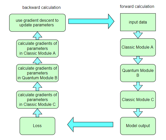
Training and testing
For the hybrid neural network model as shown in the figure below, we calculate the loss function by feeding data into the model iteratively, and VQNet will calculate the gradient of each parameter in the backward calculation automatically, and use the optimizer to optimize the parameters until the number of iterations meets the preset value.
x_train, y_train, x_test, y_test = data_select(1000, 100)

#Create a model
model = Net()
#Use adam optimizer
optimizer = Adam(model.parameters(), lr=0.005)
#Use cross entropy loss
loss_func = CategoricalCrossEntropy()

#train epoches
epochs = 10
train_loss_list = []
val_loss_list = []
train_acc_list =[]
val_acc_list = []


for epoch in range(1, epochs):
    total_loss = []
    model.train()
    batch_size = 1
    correct = 0
    n_train = 0
    for x, y in data_generator(x_train, y_train, batch_size=1, shuffle=True):

        x = x.reshape(-1, 1, 28, 28)

        optimizer.zero_grad()
        output = model(x)
        loss = loss_func(y, output)
        loss_np = np.array(loss.data)

        np_output = np.array(output.data, copy=False)
        mask = (np_output.argmax(1) == y.argmax(1))
        correct += np.sum(np.array(mask))
        n_train += batch_size

        loss.backward()
        optimizer._step()

        total_loss.append(loss_np)

    train_loss_list.append(np.sum(total_loss) / len(total_loss))
    train_acc_list.append(np.sum(correct) / n_train)
    print("{:.0f} loss is : {:.10f}".format(epoch, train_loss_list[-1]))


    model.eval()
    correct = 0
    n_eval = 0

    for x, y in data_generator(x_test, y_test, batch_size=1, shuffle=True):
        x = x.reshape(-1, 1, 28, 28)
        output = model(x)
        loss = loss_func(y, output)
        loss_np = np.array(loss.data)
        np_output = np.array(output.data, copy=False)
        mask = (np_output.argmax(1) == y.argmax(1))
        correct += np.sum(np.array(mask))
        n_eval += 1

        total_loss.append(loss_np)
    print(f"Eval Accuracy: {correct / n_eval}")
    val_loss_list.append(np.sum(total_loss) / len(total_loss))
    val_acc_list.append(np.sum(correct) / n_eval)
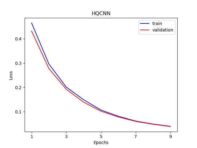
Visualization
The visualization curve of data loss function and accuracy on train and test data.
import os
plt.figure()
xrange = range(1,len(train_loss_list)+1)
figure_path = os.path.join(os.getcwd(), 'HQCNN LOSS.png')
plt.plot(xrange,train_loss_list, color="blue", label="train")
plt.plot(xrange,val_loss_list, color="red", label="validation")
plt.title('HQCNN')
plt.xlabel("Epochs")
plt.ylabel("Loss")
plt.xticks(np.arange(1, epochs +1,step = 2))
plt.legend(loc="upper right")
plt.savefig(figure_path)
plt.show()

plt.figure()
figure_path = os.path.join(os.getcwd(), 'HQCNN Accuracy.png')
plt.plot(xrange,train_acc_list, color="blue", label="train")
plt.plot(xrange,val_acc_list, color="red", label="validation")
plt.title('HQCNN')
plt.xlabel("Epochs")
plt.ylabel("Accuracy")
plt.xticks(np.arange(1, epochs +1,step = 2))
plt.legend(loc="lower right")
plt.savefig(figure_path)
plt.show()
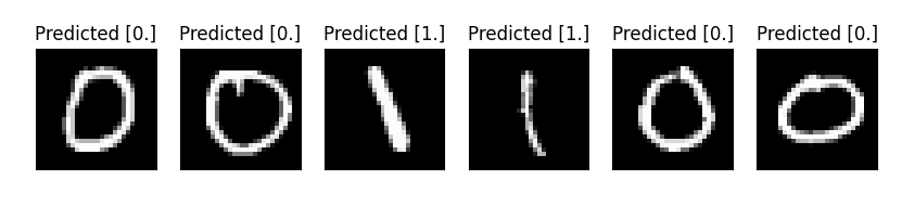
n_samples_show = 6
count = 0
fig, axes = plt.subplots(nrows=1, ncols=n_samples_show, figsize=(10, 3))
model.eval()
for x, y in data_generator(x_test, y_test, batch_size=1, shuffle=True):
    if count == n_samples_show:
        break
    x = x.reshape(-1, 1, 28, 28)
    output = model(x)
    pred = QTensor.argmax(output, [1],False)
    axes[count].imshow(x[0].squeeze(), cmap='gray')
    axes[count].set_xticks([])
    axes[count].set_yticks([])
    axes[count].set_title('Predicted {}'.format(np.array(pred.data)))
    count += 1
plt.show()
2.Hybrid quantum classical transfer learning model
We apply a machine learning method called transfer learning to image classifier based on hybrid classical quantum network. We will write a simple example of integrating pyQPanda2 with VQNet.Transfer learning is based on general intuition, that is, if the pre-trained network is good at solving a given problem, it can also be used to solve a different but related problem with only some additional training.
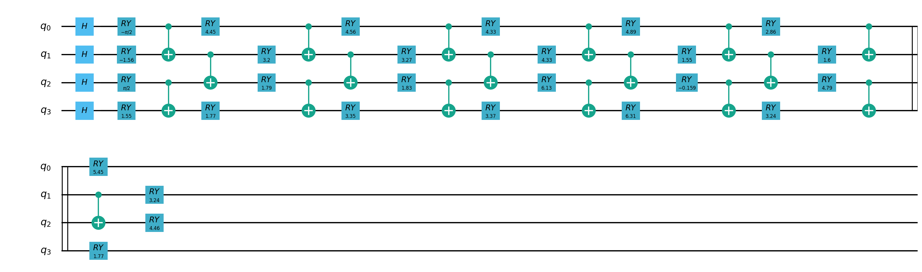
Quantum partial circuit diagram are illustrated below:
"""
Quantum Classic Nerual Network Transfer Learning demo

"""

import os
import sys
sys.path.insert(0,'../')
import numpy as np
import matplotlib.pyplot as plt

from pyvqnet.nn.module import Module
from pyvqnet.nn.linear import Linear
from pyvqnet.nn.conv import Conv2D
from pyvqnet.utils.storage import load_parameters, save_parameters

from pyvqnet.nn import activation as F
from pyvqnet.nn.pooling import MaxPool2D

from pyvqnet.nn.batch_norm import BatchNorm2d
from pyvqnet.nn.loss import SoftmaxCrossEntropy

from pyvqnet.optim.sgd import SGD
from pyvqnet.optim.adam import Adam
from pyvqnet.data.data import data_generator
from pyvqnet.tensor import tensor
from pyvqnet.tensor.tensor import QTensor
import pyqpanda as pq
from pyqpanda import *
import matplotlib
from pyvqnet.nn.module import *
from pyvqnet.utils.initializer import *
from pyvqnet.qnn.quantumlayer import QuantumLayer

try:
    matplotlib.use('TkAgg')
except:
    pass

try:
    import urllib.request
except ImportError:
    raise ImportError('You should use Python 3.x')
import os.path
import gzip

url_base = 'https://ossci-datasets.s3.amazonaws.com/mnist/'
key_file = {
    'train_img':'train-images-idx3-ubyte.gz',
    'train_label':'train-labels-idx1-ubyte.gz',
    'test_img':'t10k-images-idx3-ubyte.gz',
    'test_label':'t10k-labels-idx1-ubyte.gz'
}

def _download(dataset_dir,file_name):
    file_path = dataset_dir + "/" + file_name

    if os.path.exists(file_path):
        with gzip.GzipFile(file_path) as f:
            file_path_ungz = file_path[:-3].replace('\\', '/')
            if not os.path.exists(file_path_ungz):
                open(file_path_ungz,"wb").write(f.read())
        return

    print("Downloading " + file_name + " ... ")
    urllib.request.urlretrieve(url_base + file_name, file_path)
    if os.path.exists(file_path):
            with gzip.GzipFile(file_path) as f:
                file_path_ungz = file_path[:-3].replace('\\', '/')
                file_path_ungz = file_path_ungz.replace('-idx', '.idx')
                if not os.path.exists(file_path_ungz):
                    open(file_path_ungz,"wb").write(f.read())
    print("Done")

def download_mnist(dataset_dir):
    for v in key_file.values():
        _download(dataset_dir,v)


if not os.path.exists("./result"):
    os.makedirs("./result")
else:
    pass
# classical CNN
class CNN(Module):
    def __init__(self):
        super(CNN, self).__init__()

        self.conv1 = Conv2D(input_channels=1, output_channels=16, kernel_size=(3, 3), stride=(1, 1), padding="valid")
        self.BatchNorm2d1 = BatchNorm2d(16)
        self.Relu1 = F.ReLu()

        self.conv2 = Conv2D(input_channels=16, output_channels=32, kernel_size=(3, 3), stride=(1, 1), padding="valid")
        self.BatchNorm2d2 = BatchNorm2d(32)
        self.Relu2 = F.ReLu()
        self.maxpool2 = MaxPool2D([2, 2], [2, 2], padding="valid")

        self.conv3 = Conv2D(input_channels=32, output_channels=64, kernel_size=(3, 3), stride=(1, 1), padding="valid")
        self.BatchNorm2d3 = BatchNorm2d(64)
        self.Relu3 = F.ReLu()

        self.conv4 = Conv2D(input_channels=64, output_channels=128, kernel_size=(3, 3), stride=(1, 1), padding="valid")
        self.BatchNorm2d4 = BatchNorm2d(128)
        self.Relu4 = F.ReLu()
        self.maxpool4 = MaxPool2D([2, 2], [2, 2], padding="valid")

        self.fc1 = Linear(input_channels=128 * 4 * 4, output_channels=1024)
        self.fc2 = Linear(input_channels=1024, output_channels=128)
        self.fc3 = Linear(input_channels=128, output_channels=10)

    def forward(self, x):

        x = self.Relu1(self.conv1(x))
        x = self.maxpool2(self.Relu2(self.conv2(x)))
        x = self.Relu3(self.conv3(x))
        x = self.maxpool4(self.Relu4(self.conv4(x)))
        x = tensor.flatten(x, 1)
        x = F.ReLu()(self.fc1(x))  # 1 64
        x = F.ReLu()(self.fc2(x))  # 1 64
        x = self.fc3(x)  # 1 1
        return x

def load_mnist(dataset="training_data", digits=np.arange(2), path="./"):
    import os, struct
    from array import array as pyarray
    download_mnist(path)
    if dataset == "training_data":
        fname_image = os.path.join(path, 'train-images.idx3-ubyte').replace('\\', '/')
        fname_label = os.path.join(path, 'train-labels.idx1-ubyte').replace('\\', '/')
    elif dataset == "testing_data":
        fname_image = os.path.join(path, 't10k-images.idx3-ubyte').replace('\\', '/')
        fname_label = os.path.join(path, 't10k-labels.idx1-ubyte').replace('\\', '/')
    else:
        raise ValueError("dataset must be 'training_data' or 'testing_data'")

    flbl = open(fname_label, 'rb')
    magic_nr, size = struct.unpack(">II", flbl.read(8))
    lbl = pyarray("b", flbl.read())
    flbl.close()

    fimg = open(fname_image, 'rb')
    magic_nr, size, rows, cols = struct.unpack(">IIII", fimg.read(16))
    img = pyarray("B", fimg.read())
    fimg.close()

    ind = [k for k in range(size) if lbl[k] in digits]
    N = len(ind)
    images = np.zeros((N, rows, cols))
    labels = np.zeros((N, 1), dtype=int)
    for i in range(len(ind)):
        images[i] = np.array(img[ind[i] * rows * cols: (ind[i] + 1) * rows * cols]).reshape((rows, cols))
        labels[i] = lbl[ind[i]]

    return images, labels


"""
to get cnn model parameters for transfer learning
"""

train_size = 10000
eval_size = 1000
EPOCHES = 100
def classcal_cnn_model_making():
    # load train data
    x_train, y_train = load_mnist("training_data", digits=np.arange(10))
    x_test, y_test = load_mnist("testing_data", digits=np.arange(10))

    x_train = x_train[:train_size]
    y_train = y_train[:train_size]
    x_test = x_test[:eval_size]
    y_test = y_test[:eval_size]

    x_train = x_train / 255
    x_test = x_test / 255
    y_train = np.eye(10)[y_train].reshape(-1, 10)
    y_test = np.eye(10)[y_test].reshape(-1, 10)

    model = CNN()

    optimizer = SGD(model.parameters(), lr=0.005)
    loss_func = SoftmaxCrossEntropy()

    epochs = EPOCHES
    loss_list = []
    model.train()

    SAVE_FLAG = True
    temp_loss = 0
    for epoch in range(1, epochs):
        total_loss = []
        for x, y in data_generator(x_train, y_train, batch_size=4, shuffle=True):

            x = x.reshape(-1, 1, 28, 28)
            optimizer.zero_grad()
            # Forward pass
            output = model(x)

            # Calculating loss
            loss = loss_func(y, output)  # target output
            loss_np = np.array(loss.data)
            # Backward pass
            loss.backward()
            # Optimize the weights
            optimizer._step()

            total_loss.append(loss_np)

        loss_list.append(np.sum(total_loss) / len(total_loss))
        print("{:.0f} loss is : {:.10f}".format(epoch, loss_list[-1]))

        if SAVE_FLAG:
            temp_loss = loss_list[-1]
            save_parameters(model.state_dict(), "./result/QCNN_TL_1.model")
            SAVE_FLAG = False
        else:
            if temp_loss > loss_list[-1]:
                temp_loss = loss_list[-1]
                save_parameters(model.state_dict(), "./result/QCNN_TL_1.model")


    model.eval()
    correct = 0
    n_eval = 0

    for x, y in data_generator(x_test, y_test, batch_size=4, shuffle=True):
        x = x.reshape(-1, 1, 28, 28)
        output = model(x)
        loss = loss_func(y, output)
        np_output = np.array(output.data, copy=False)
        mask = (np_output.argmax(1) == y.argmax(1))
        correct += np.sum(np.array(mask))
        n_eval += 1
    print(f"Eval Accuracy: {correct / n_eval}")

    n_samples_show = 6
    count = 0
    fig, axes = plt.subplots(nrows=1, ncols=n_samples_show, figsize=(10, 3))
    model.eval()
    for x, y in data_generator(x_test, y_test, batch_size=1, shuffle=True):
        if count == n_samples_show:
            break
        x = x.reshape(-1, 1, 28, 28)
        output = model(x)
        pred = QTensor.argmax(output, [1],False)
        axes[count].imshow(x[0].squeeze(), cmap='gray')
        axes[count].set_xticks([])
        axes[count].set_yticks([])
        axes[count].set_title('Predicted {}'.format(np.array(pred.data)))
        count += 1
    plt.show()

def classical_cnn_TransferLearning_predict():
    x_test, y_test = load_mnist("testing_data", digits=np.arange(10))

    x_test = x_test[:eval_size]
    y_test = y_test[:eval_size]
    x_test = x_test / 255
    y_test = np.eye(10)[y_test].reshape(-1, 10)
    model = CNN()

    model_parameter = load_parameters("./result/QCNN_TL_1.model")
    model.load_state_dict(model_parameter)
    model.eval()
    correct = 0
    n_eval = 0

    for x, y in data_generator(x_test, y_test, batch_size=1, shuffle=True):
        x = x.reshape(-1, 1, 28, 28)
        output = model(x)

        np_output = np.array(output.data, copy=False)
        mask = (np_output.argmax(1) == y.argmax(1))
        correct += np.sum(np.array(mask))
        n_eval += 1

    print(f"Eval Accuracy: {correct / n_eval}")

    n_samples_show = 6
    count = 0
    fig, axes = plt.subplots(nrows=1, ncols=n_samples_show, figsize=(10, 3))
    model.eval()
    for x, y in data_generator(x_test, y_test, batch_size=1, shuffle=True):
        if count == n_samples_show:
            break
        x = x.reshape(-1, 1, 28, 28)
        output = model(x)
        pred = QTensor.argmax(output, [1],False)
        axes[count].imshow(x[0].squeeze(), cmap='gray')
        axes[count].set_xticks([])
        axes[count].set_yticks([])
        axes[count].set_title('Predicted {}'.format(np.array(pred.data)))
        count += 1
    plt.show()

def quantum_cnn_TransferLearning():

    n_qubits = 4  # Number of qubits
    q_depth = 6  # Depth of the quantum circuit (number of variational layers)

    def Q_H_layer(qubits, nqubits):
        """Layer of single-qubit Hadamard gates.
        """
        circuit = pq.QCircuit()
        for idx in range(nqubits):
            circuit.insert(pq.H(qubits[idx]))
        return circuit

    def Q_RY_layer(qubits, w):
        """Layer of parametrized qubit rotations around the y axis.
        """
        circuit = pq.QCircuit()
        for idx, element in enumerate(w):
            circuit.insert(pq.RY(qubits[idx], element))
        return circuit

    def Q_entangling_layer(qubits, nqubits):
        """Layer of CNOTs followed by another shifted layer of CNOT.
        """
        # In other words it should apply something like :
        # CNOT  CNOT  CNOT  CNOT...  CNOT
        #   CNOT  CNOT  CNOT...  CNOT
        circuit = pq.QCircuit()
        for i in range(0, nqubits - 1, 2):  # Loop over even indices: i=0,2,...N-2
            circuit.insert(pq.CNOT(qubits[i], qubits[i + 1]))
        for i in range(1, nqubits - 1, 2):  # Loop over odd indices:  i=1,3,...N-3
            circuit.insert(pq.CNOT(qubits[i], qubits[i + 1]))
        return circuit

    def Q_quantum_net(q_input_features, q_weights_flat, qubits, cubits, machine):
        """
        The variational quantum circuit.
        """
        machine = pq.CPUQVM()
        machine.init_qvm()
        qubits = machine.qAlloc_many(n_qubits)
        circuit = pq.QCircuit()

        # Reshape weights
        q_weights = q_weights_flat.reshape([q_depth, n_qubits])

        # Start from state |+> , unbiased w.r.t. |0> and |1>
        circuit.insert(Q_H_layer(qubits, n_qubits))

        # Embed features in the quantum node
        circuit.insert(Q_RY_layer(qubits, q_input_features))

        # Sequence of trainable variational layers
        for k in range(q_depth):
            circuit.insert(Q_entangling_layer(qubits, n_qubits))
            circuit.insert(Q_RY_layer(qubits, q_weights[k]))

        # Expectation values in the Z basis
        prog = pq.QProg()
        prog.insert(circuit)

        exp_vals = []
        for position in range(n_qubits):
            pauli_str = "Z" + str(position)
            pauli_map = pq.PauliOperator(pauli_str, 1)
            hamiltion = pauli_map.toHamiltonian(True)
            exp = machine.get_expectation(prog, hamiltion, qubits)
            exp_vals.append(exp)

        return exp_vals

    class Q_DressedQuantumNet(Module):

        def __init__(self):
            """
            Definition of the *dressed* layout.
            """

            super().__init__()
            self.pre_net = Linear(128, n_qubits)
            self.post_net = Linear(n_qubits, 10)
            self.temp_Q = QuantumLayer(Q_quantum_net, q_depth * n_qubits, "cpu", n_qubits, n_qubits)

        def forward(self, input_features):
            """
            Defining how tensors are supposed to move through the *dressed* quantum
            net.
            """

            # obtain the input features for the quantum circuit
            # by reducing the feature dimension from 512 to 4
            pre_out = self.pre_net(input_features)
            q_in = tensor.tanh(pre_out) * np.pi / 2.0
            q_out_elem = self.temp_Q(q_in)

            result = q_out_elem
            # return the two-dimensional prediction from the postprocessing layer
            return self.post_net(result)

    x_train, y_train = load_mnist("training_data", digits=np.arange(10))
    x_test, y_test = load_mnist("testing_data", digits=np.arange(10))
    x_train = x_train[:train_size]
    y_train = y_train[:train_size]
    x_test = x_test[:eval_size]
    y_test = y_test[:eval_size]

    x_train = x_train / 255
    x_test = x_test / 255
    y_train = np.eye(10)[y_train].reshape(-1, 10)
    y_test = np.eye(10)[y_test].reshape(-1, 10)

    model = CNN()
    model_param = load_parameters("./result/QCNN_TL_1.model")
    model.load_state_dict(model_param)

    loss_func = SoftmaxCrossEntropy()

    epochs = EPOCHES
    loss_list = []
    eval_losses = []

    model_hybrid = model
    print(model_hybrid)

    for param in model_hybrid.parameters():
        param.requires_grad = False
    model_hybrid.fc3 = Q_DressedQuantumNet()
    optimizer_hybrid = Adam(model_hybrid.fc3.parameters(), lr=0.001)
    model_hybrid.train()

    SAVE_FLAG = True
    temp_loss = 0
    for epoch in range(1, epochs):
        total_loss = []
        for x, y in data_generator(x_train, y_train, batch_size=4, shuffle=True):
            x = x.reshape(-1, 1, 28, 28)
            optimizer_hybrid.zero_grad()
            # Forward pass
            output = model_hybrid(x)

            loss = loss_func(y, output)  # target output
            loss_np = np.array(loss.data)
            # Backward pass
            loss.backward()
            # Optimize the weights
            optimizer_hybrid._step()
            total_loss.append(loss_np)

        loss_list.append(np.sum(total_loss) / len(total_loss))
        print("{:.0f} loss is : {:.10f}".format(epoch, loss_list[-1]))
        if SAVE_FLAG:
            temp_loss = loss_list[-1]
            save_parameters(model_hybrid.fc3.state_dict(), "./result/QCNN_TL_FC3.model")
            save_parameters(model_hybrid.state_dict(), "./result/QCNN_TL_ALL.model")
            SAVE_FLAG = False
        else:
            if temp_loss > loss_list[-1]:
                temp_loss = loss_list[-1]
                save_parameters(model_hybrid.fc3.state_dict(), "./result/QCNN_TL_FC3.model")
                save_parameters(model_hybrid.state_dict(), "./result/QCNN_TL_ALL.model")

        correct = 0
        n_eval = 0
        loss_temp =[]
        for x1, y1 in data_generator(x_test, y_test, batch_size=4, shuffle=True):
            x1 = x1.reshape(-1, 1, 28, 28)
            output = model_hybrid(x1)
            loss = loss_func(y1, output)
            np_loss = np.array(loss.data)
            np_output = np.array(output.data, copy=False)
            mask = (np_output.argmax(1) == y1.argmax(1))
            correct += np.sum(np.array(mask))
            n_eval += 1
            loss_temp.append(np_loss)
        eval_losses.append(np.sum(loss_temp) / n_eval)
        print("{:.0f} eval loss is : {:.10f}".format(epoch, eval_losses[-1]))


    plt.title('model loss')
    plt.plot(loss_list, color='green', label='train_losses')
    plt.plot(eval_losses, color='red', label='eval_losses')
    plt.ylabel('loss')
    plt.legend(["train_losses", "eval_losses"])
    plt.savefig("qcnn_transfer_learning_classical")
    plt.show()
    plt.close()

    n_samples_show = 6
    count = 0
    fig, axes = plt.subplots(nrows=1, ncols=n_samples_show, figsize=(10, 3))
    model_hybrid.eval()
    for x, y in data_generator(x_test, y_test, batch_size=1, shuffle=True):
        if count == n_samples_show:
            break
        x = x.reshape(-1, 1, 28, 28)
        output = model_hybrid(x)
        pred = QTensor.argmax(output, [1],False)
        axes[count].imshow(x[0].squeeze(), cmap='gray')
        axes[count].set_xticks([])
        axes[count].set_yticks([])
        axes[count].set_title('Predicted {}'.format(np.array(pred.data)))
        count += 1
    plt.show()

def quantum_cnn_TransferLearning_predict():

    n_qubits = 4  # Number of qubits
    q_depth = 6  # Depth of the quantum circuit (number of variational layers)

    def Q_H_layer(qubits, nqubits):
        """Layer of single-qubit Hadamard gates.
        """
        circuit = pq.QCircuit()
        for idx in range(nqubits):
            circuit.insert(pq.H(qubits[idx]))
        return circuit

    def Q_RY_layer(qubits, w):
        """Layer of parametrized qubit rotations around the y axis.
        """
        circuit = pq.QCircuit()
        for idx, element in enumerate(w):
            circuit.insert(pq.RY(qubits[idx], element))
        return circuit

    def Q_entangling_layer(qubits, nqubits):
        """Layer of CNOTs followed by another shifted layer of CNOT.
        """
        # In other words it should apply something like :
        # CNOT  CNOT  CNOT  CNOT...  CNOT
        #   CNOT  CNOT  CNOT...  CNOT
        circuit = pq.QCircuit()
        for i in range(0, nqubits - 1, 2):  # Loop over even indices: i=0,2,...N-2
            circuit.insert(pq.CNOT(qubits[i], qubits[i + 1]))
        for i in range(1, nqubits - 1, 2):  # Loop over odd indices:  i=1,3,...N-3
            circuit.insert(pq.CNOT(qubits[i], qubits[i + 1]))
        return circuit

    def Q_quantum_net(q_input_features, q_weights_flat, qubits, cubits, machine):
        """
        The variational quantum circuit.
        """
        machine = pq.CPUQVM()
        machine.init_qvm()
        qubits = machine.qAlloc_many(n_qubits)
        circuit = pq.QCircuit()

        # Reshape weights
        q_weights = q_weights_flat.reshape([q_depth, n_qubits])

        # Start from state |+> , unbiased w.r.t. |0> and |1>
        circuit.insert(Q_H_layer(qubits, n_qubits))

        # Embed features in the quantum node
        circuit.insert(Q_RY_layer(qubits, q_input_features))

        # Sequence of trainable variational layers
        for k in range(q_depth):
            circuit.insert(Q_entangling_layer(qubits, n_qubits))
            circuit.insert(Q_RY_layer(qubits, q_weights[k]))

        # Expectation values in the Z basis
        prog = pq.QProg()
        prog.insert(circuit)
        exp_vals = []
        for position in range(n_qubits):
            pauli_str = "Z" + str(position)
            pauli_map = pq.PauliOperator(pauli_str, 1)
            hamiltion = pauli_map.toHamiltonian(True)
            exp = machine.get_expectation(prog, hamiltion, qubits)
            exp_vals.append(exp)

        return exp_vals

    class Q_DressedQuantumNet(Module):

        def __init__(self):
            """
            Definition of the *dressed* layout.
            """

            super().__init__()
            self.pre_net = Linear(128, n_qubits)
            self.post_net = Linear(n_qubits, 10)
            self.temp_Q = QuantumLayer(Q_quantum_net, q_depth * n_qubits, "cpu", n_qubits, n_qubits)

        def forward(self, input_features):
            """
            Defining how tensors are supposed to move through the *dressed* quantum
            net.
            """

            # obtain the input features for the quantum circuit
            # by reducing the feature dimension from 512 to 4
            pre_out = self.pre_net(input_features)
            q_in = tensor.tanh(pre_out) * np.pi / 2.0
            q_out_elem = self.temp_Q(q_in)

            result = q_out_elem
            # return the two-dimensional prediction from the postprocessing layer
            return self.post_net(result)

    x_train, y_train = load_mnist("training_data", digits=np.arange(10))
    x_test, y_test = load_mnist("testing_data", digits=np.arange(10))
    x_train = x_train[:2000]
    y_train = y_train[:2000]
    x_test = x_test[:500]
    y_test = y_test[:500]

    x_train = x_train / 255
    x_test = x_test / 255
    y_train = np.eye(10)[y_train].reshape(-1, 10)
    y_test = np.eye(10)[y_test].reshape(-1, 10)

    model = CNN()
    model_hybrid = model
    model_hybrid.fc3 = Q_DressedQuantumNet()
    for param in model_hybrid.parameters():
        param.requires_grad = False
    model_param_quantum = load_parameters("./result/QCNN_TL_ALL.model")

    model_hybrid.load_state_dict(model_param_quantum)
    model_hybrid.eval()

    loss_func = SoftmaxCrossEntropy()
    eval_losses = []

    correct = 0
    n_eval = 0
    loss_temp =[]
    eval_batch_size = 4
    for x1, y1 in data_generator(x_test, y_test, batch_size=eval_batch_size, shuffle=True):
        x1 = x1.reshape(-1, 1, 28, 28)
        output = model_hybrid(x1)
        loss = loss_func(y1, output)
        np_loss = np.array(loss.data)
        np_output = np.array(output.data, copy=False)
        mask = (np_output.argmax(1) == y1.argmax(1))
        correct += np.sum(np.array(mask))

        n_eval += 1
        loss_temp.append(np_loss)

    eval_losses.append(np.sum(loss_temp) / n_eval)
    print(f"Eval Accuracy: {correct / (eval_batch_size*n_eval)}")

    n_samples_show = 6
    count = 0
    fig, axes = plt.subplots(nrows=1, ncols=n_samples_show, figsize=(10, 3))
    model_hybrid.eval()
    for x, y in data_generator(x_test, y_test, batch_size=1, shuffle=True):
        if count == n_samples_show:
            break
        x = x.reshape(-1, 1, 28, 28)
        output = model_hybrid(x)
        pred = QTensor.argmax(output, [1],False)
        axes[count].imshow(x[0].squeeze(), cmap='gray')
        axes[count].set_xticks([])
        axes[count].set_yticks([])
        axes[count].set_title('Predicted {}'.format(np.array(pred.data)))
        count += 1
    plt.show()

if __name__ == "__main__":
    # save classic model parameters
    if not os.path.exists('./result/QCNN_TL_1.model'):
        classcal_cnn_model_making()
        classical_cnn_TransferLearning_predict()
    #train quantum circuits.
    print("use exist cnn model param to train quantum parameters.")
    quantum_cnn_TransferLearning()
    #eval quantum circuits.
    quantum_cnn_TransferLearning_predict()
Loss on training set
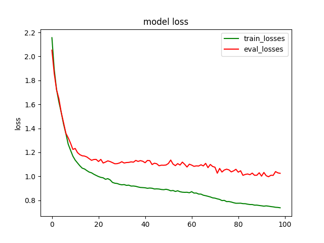
Run classification on test set
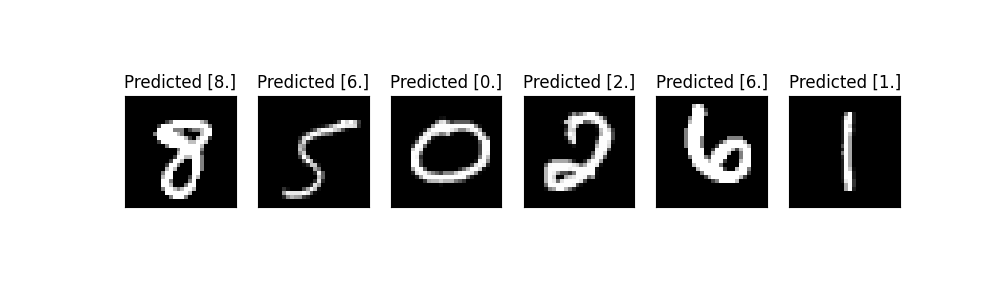
3. Hybrid quantum classical Unet network model
Image segmentation Image segmentation is a classical problem in the research of computer vision and has become a hot spot in the field of image understanding. Image segmentation an important part of image understanding, and one of the most difficult problems in image processing. The so-called image segmentation refers to the segmentation based on gray, color and spatial texture The image is divided into several disjoint regions by features such as theory and geometry, so that these features show consistency or similarity in the same region and obvious differences between different regions. In short, it is to give a picture and classify each pixel on the picture. Separate the pixel regions belonging to different objects. Unet is a classical image segmentation algorithm.
Here, we explore how to partially quantify the classical neural network to create a hybrid quantum classical QUnet neural network. We will write a simple example of integrating pyQPanda2 with VQNet . Qunet is mainly used to solve the technology of image segmentation.
Data preparation
We will use the data of VOC2012 official library as image segmentation data. These samples are divided into training data training_data and test data testing_data.
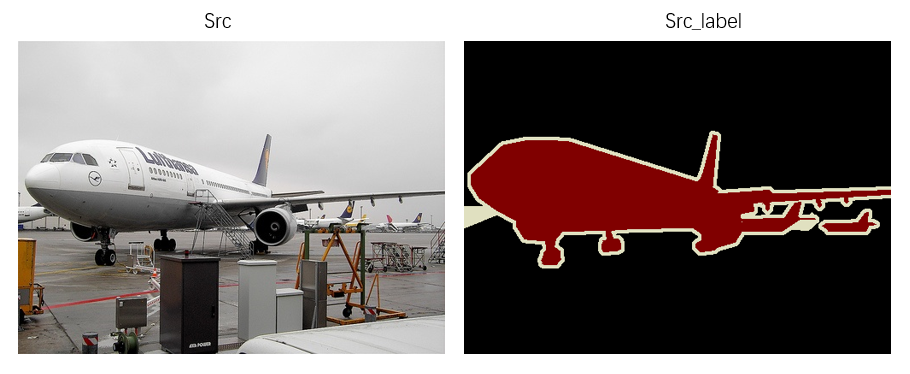
Constructing quantum circuits
In this example, we define a quantum circuit using pyqpanda2. The input 3-channel color image data is compressed into a single channel gray image and stored, and then the feature of the data is extracted and dimensionality reduced by quantum convolution operation.
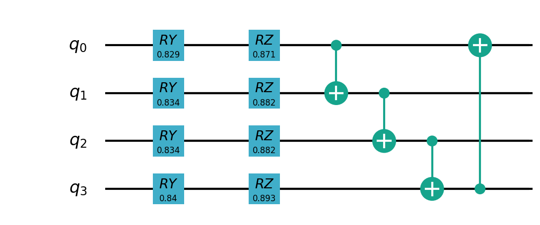
Import necessary libraries and functions
import os
import numpy as np
from pyvqnet.nn.module import Module
from pyvqnet.nn.conv import Conv2D, ConvT2D
from pyvqnet.nn import activation as F
from pyvqnet.nn.batch_norm import BatchNorm2d
from pyvqnet.nn.loss import BinaryCrossEntropy
from pyvqnet.optim.adam import Adam
from pyvqnet.dtype import *
from pyvqnet.tensor import tensor,kfloat32
from pyvqnet.tensor.tensor import QTensor
import pyqpanda as pq
from pyqpanda import *
from pyvqnet.utils.storage import load_parameters, save_parameters

import matplotlib
try:
    matplotlib.use('TkAgg')
except:
    pass
import matplotlib.pyplot as plt

import cv2
Preprocessing data
# Preprocessing data
class PreprocessingData:
    def __init__(self, path):
        self.path = path
        self.x_data = []
        self.y_label = []


    def processing(self):
        list_path = os.listdir((self.path+"/images"))
        for i in range(len(list_path)):

            temp_data = cv2.imread(self.path+"/images" + '/' + list_path[i], cv2.IMREAD_COLOR)
            temp_data = cv2.resize(temp_data, (128, 128))
            grayimg = cv2.cvtColor(temp_data, cv2.COLOR_BGR2GRAY)
            temp_data = grayimg.reshape(temp_data.shape[0], temp_data.shape[0], 1).astype(np.float32)
            self.x_data.append(temp_data)

            label_data = cv2.imread(self.path+"/labels" + '/' +list_path[i].split(".")[0] + ".png", cv2.IMREAD_COLOR)
            label_data = cv2.resize(label_data, (128, 128))

            label_data = cv2.cvtColor(label_data, cv2.COLOR_BGR2GRAY)
            label_data = label_data.reshape(label_data.shape[0], label_data.shape[0], 1).astype(np.int64)
            self.y_label.append(label_data)

        return self.x_data, self.y_label

    def read(self):
        self.x_data, self.y_label = self.processing()
        x_data = np.array(self.x_data)
        y_label = np.array(self.y_label)

        return x_data, y_label

# Quantum coding circuit
class QCNN_:
    def __init__(self, image):
        self.image = image

    def encode_cir(self, qlist, pixels):
        cir = pq.QCircuit()
        for i, pix in enumerate(pixels):
            theta = np.arctan(pix)
            phi = np.arctan(pix**2)
            cir.insert(pq.RY(qlist[i], theta))
            cir.insert(pq.RZ(qlist[i], phi))
        return cir

    def entangle_cir(self, qlist):
        k_size = len(qlist)
        cir = pq.QCircuit()
        for i in range(k_size):
            ctr = i
            ctred = i+1
            if ctred == k_size:
                ctred = 0
            cir.insert(pq.CNOT(qlist[ctr], qlist[ctred]))
        return cir

    def qcnn_circuit(self, pixels):
        k_size = len(pixels)
        machine = pq.MPSQVM()
        machine.init_qvm()
        qlist = machine.qAlloc_many(k_size)
        cir = pq.QProg()

        cir.insert(self.encode_cir(qlist, np.array(pixels) * np.pi / 2))
        cir.insert(self.entangle_cir(qlist))

        result0 = machine.prob_run_list(cir, [qlist[0]], -1)
        result1 = machine.prob_run_list(cir, [qlist[1]], -1)
        result2 = machine.prob_run_list(cir, [qlist[2]], -1)
        result3 = machine.prob_run_list(cir, [qlist[3]], -1)

        result = [result0[-1]+result1[-1]+result2[-1]+result3[-1]]
        machine.finalize()
        return result

def quanconv_(image):
    """Convolves the input image with many applications of the same quantum circuit."""
    out = np.zeros((64, 64, 1))

    for j in range(0, 128, 2):
        for k in range(0, 128, 2):
            # Process a squared 2x2 region of the image with a quantum circuit
            q_results = QCNN_(image).qcnn_circuit(
                [
                    image[j, k, 0],
                    image[j, k + 1, 0],
                    image[j + 1, k, 0],
                    image[j + 1, k + 1, 0]
                ]
            )

            for c in range(1):
                out[j // 2, k // 2, c] = q_results[c]
    return out

def quantum_data_preprocessing(images):
    quantum_images = []
    for _, img in enumerate(images):
        quantum_images.append(quanconv_(img))
    quantum_images = np.asarray(quantum_images)
    return quantum_images
Constructing hybrid classical quantum neural network
According to the Unet network framework, we use the VQNet framework to build the classic network part. The down-sampling neural network layer is used to reduce the dimension and extract features; The up-sampling neural network layer is used to restore the dimension; The up and down sampling layers are connected through concatenate for feature fusion.
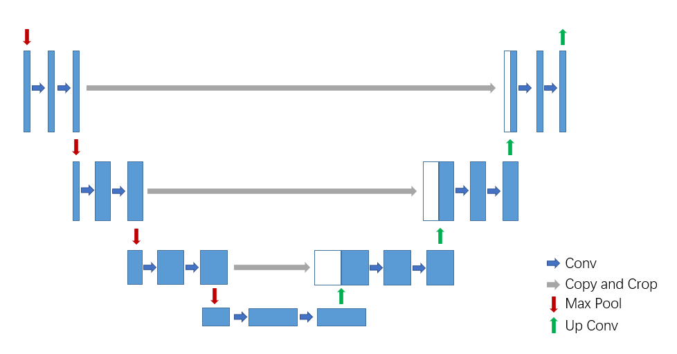
# Definition of down sampling neural network layer
class DownsampleLayer(Module):
    def __init__(self, in_ch, out_ch):
        super(DownsampleLayer, self).__init__()
        self.conv1 = Conv2D(input_channels=in_ch, output_channels=out_ch, kernel_size=(3, 3), stride=(1, 1),
                            padding="same")
        self.BatchNorm2d1 = BatchNorm2d(out_ch)
        self.Relu1 = F.ReLu()
        self.conv2 = Conv2D(input_channels=out_ch, output_channels=out_ch, kernel_size=(3, 3), stride=(1, 1),
                            padding="same")
        self.BatchNorm2d2 = BatchNorm2d(out_ch)
        self.Relu2 = F.ReLu()
        self.conv3 = Conv2D(input_channels=out_ch, output_channels=out_ch, kernel_size=(3, 3), stride=(2, 2),
                            padding=(1,1))
        self.BatchNorm2d3 = BatchNorm2d(out_ch)
        self.Relu3 = F.ReLu()

    def forward(self, x):
        """
        :param x:
        :return: out(Output to deep),out_2(enter to next level),
        """
        x1 = self.conv1(x)
        x2 = self.BatchNorm2d1(x1)
        x3 = self.Relu1(x2)
        x4 = self.conv2(x3)
        x5 = self.BatchNorm2d2(x4)
        out = self.Relu2(x5)
        x6 = self.conv3(out)
        x7 = self.BatchNorm2d3(x6)
        out_2 = self.Relu3(x7)
        return out, out_2

# Definition of up sampling neural network layer
class UpSampleLayer(Module):
    def __init__(self, in_ch, out_ch):
        super(UpSampleLayer, self).__init__()

        self.conv1 = Conv2D(input_channels=in_ch, output_channels=out_ch * 2, kernel_size=(3, 3), stride=(1, 1),
                            padding="same")
        self.BatchNorm2d1 = BatchNorm2d(out_ch * 2)
        self.Relu1 = F.ReLu()
        self.conv2 = Conv2D(input_channels=out_ch * 2, output_channels=out_ch * 2, kernel_size=(3, 3), stride=(1, 1),
                            padding="same")
        self.BatchNorm2d2 = BatchNorm2d(out_ch * 2)
        self.Relu2 = F.ReLu()

        self.conv3 = ConvT2D(input_channels=out_ch * 2, output_channels=out_ch, kernel_size=(3, 3), stride=(2, 2),
                             padding=(1,1))
        self.BatchNorm2d3 = BatchNorm2d(out_ch)
        self.Relu3 = F.ReLu()

    def forward(self, x):
        '''
        :param x: input conv layer
        :param out: connect with UpsampleLayer
        :return:
        '''
        x = self.conv1(x)
        x = self.BatchNorm2d1(x)
        x = self.Relu1(x)
        x = self.conv2(x)
        x = self.BatchNorm2d2(x)
        x = self.Relu2(x)
        x = self.conv3(x)
        x = self.BatchNorm2d3(x)
        x_out = self.Relu3(x)
        return x_out

# Unet overall network architecture
class UNet(Module):
    def __init__(self):
        super(UNet, self).__init__()
        out_channels = [2 ** (i + 4) for i in range(5)]

        # DownSampleLayer
        self.d1 = DownsampleLayer(1, out_channels[0])  # 3-64
        self.d2 = DownsampleLayer(out_channels[0], out_channels[1])  # 64-128
        self.d3 = DownsampleLayer(out_channels[1], out_channels[2])  # 128-256
        self.d4 = DownsampleLayer(out_channels[2], out_channels[3])  # 256-512
        # UpSampleLayer
        self.u1 = UpSampleLayer(out_channels[3], out_channels[3])  # 512-1024-512
        self.u2 = UpSampleLayer(out_channels[4], out_channels[2])  # 1024-512-256
        self.u3 = UpSampleLayer(out_channels[3], out_channels[1])  # 512-256-128
        self.u4 = UpSampleLayer(out_channels[2], out_channels[0])  # 256-128-64
        # output
        self.conv1 = Conv2D(input_channels=out_channels[1], output_channels=out_channels[0], kernel_size=(3, 3),
                            stride=(1, 1), padding="same")
        self.BatchNorm2d1 = BatchNorm2d(out_channels[0])
        self.Relu1 = F.ReLu()
        self.conv2 = Conv2D(input_channels=out_channels[0], output_channels=out_channels[0], kernel_size=(3, 3),
                            stride=(1, 1), padding="same")
        self.BatchNorm2d2 = BatchNorm2d(out_channels[0])
        self.Relu2 = F.ReLu()
        self.conv3 = Conv2D(input_channels=out_channels[0], output_channels=1, kernel_size=(3, 3),
                            stride=(1, 1), padding="same")
        self.Sigmoid = F.Sigmoid()

    def forward(self, x):
        out_1, out1 = self.d1(x)
        out_2, out2 = self.d2(out1)
        out_3, out3 = self.d3(out2)
        out_4, out4 = self.d4(out3)

        out5 = self.u1(out4)
        out5_pad_out4 = tensor.pad2d(out5, (1, 0, 1, 0), 0)
        cat_out5 = tensor.concatenate([out5_pad_out4, out_4], axis=1)

        out6 = self.u2(cat_out5)
        out6_pad_out_3 = tensor.pad2d(out6, (1, 0, 1, 0), 0)
        cat_out6 = tensor.concatenate([out6_pad_out_3, out_3], axis=1)

        out7 = self.u3(cat_out6)
        out7_pad_out_2 = tensor.pad2d(out7, (1, 0, 1, 0), 0)
        cat_out7 = tensor.concatenate([out7_pad_out_2, out_2], axis=1)

        out8 = self.u4(cat_out7)
        out8_pad_out_1 = tensor.pad2d(out8, (1, 0, 1, 0), 0)
        cat_out8 = tensor.concatenate([out8_pad_out_1, out_1], axis=1)
        out = self.conv1(cat_out8)
        out = self.BatchNorm2d1(out)
        out = self.Relu1(out)
        out = self.conv2(out)
        out = self.BatchNorm2d2(out)
        out = self.Relu2(out)
        out = self.conv3(out)
        out = self.Sigmoid(out)
        return out
Training and model saving
Similar to the training of classical neural network model,
we also need to instantiate the model, define the loss function and optimizer, and define the whole training and
testing process. For the hybrid neural network model as shown in the figure below, we calculate the loss value in
forward function the gradient of each parameter in
reverse calculation automatically, and use the optimizer to optimize the parameters until the number of
iterations meets the preset value.If PREPROCESS is False, the code will skip the quantum data preprocessing.
PREPROCESS = True

class MyDataset():
    def __init__(self, x_data, x_label):
        self.x_set = x_data
        self.label = x_label

    def __getitem__(self, item):
        img, target = self.x_set[item], self.label[item]
        img_np = np.uint8(img).transpose(2, 0, 1)
        target_np = np.uint8(target).transpose(2, 0, 1)

        img = img_np
        target = target_np
        return img, target

    def __len__(self):
        return len(self.x_set)

if not os.path.exists("./result"):
    os.makedirs("./result")
else:
    pass
if not os.path.exists("./Intermediate_results"):
    os.makedirs("./Intermediate_results")
else:
    pass

# prepare train/test data and label
path0 = 'training_data'
path1 = 'testing_data'
train_images, train_labels = PreprocessingData(path0).read()
test_images, test_labels = PreprocessingData(path1).read()

print('train: ', train_images.shape, '\ntest: ', test_images.shape)
print('train: ', train_labels.shape, '\ntest: ', test_labels.shape)
train_images = train_images / 255
test_images = test_images / 255

# use quantum encoder to preprocess data

if PREPROCESS == True:
    print("Quantum pre-processing of train images:")
    q_train_images = quantum_data_preprocessing(train_images)
    q_test_images = quantum_data_preprocessing(test_images)
    q_train_label = quantum_data_preprocessing(train_labels)
    q_test_label = quantum_data_preprocessing(test_labels)

    # Save pre-processed images
    print('Quantum Data Saving...')
    np.save("./result/q_train.npy", q_train_images)
    np.save("./result/q_test.npy", q_test_images)
    np.save("./result/q_train_label.npy", q_train_label)
    np.save("./result/q_test_label.npy", q_test_label)
    print('Quantum Data Saving Over!')

# loading quantum data
SAVE_PATH = "./result/"
train_x = np.load(SAVE_PATH + "q_train.npy")
train_labels = np.load(SAVE_PATH + "q_train_label.npy")
test_x = np.load(SAVE_PATH + "q_test.npy")
test_labels = np.load(SAVE_PATH + "q_test_label.npy")

train_x = train_x.astype(np.uint8)
test_x = test_x.astype(np.uint8)
train_labels = train_labels.astype(np.uint8)
test_labels = test_labels.astype(np.uint8)
train_y = train_labels
test_y = test_labels

trainset = MyDataset(train_x, train_y)
testset = MyDataset(test_x, test_y)

x_train = []
y_label = []
model = UNet()
optimizer = Adam(model.parameters(), lr=0.01)
loss_func = BinaryCrossEntropy()
epochs = 200

loss_list = []
SAVE_FLAG = True
temp_loss = 0
file = open("./result/result.txt", 'w').close()
for epoch in range(1, epochs):
    total_loss = []
    model.train()
    for i, (x, y) in enumerate(trainset):
        x_img = QTensor(x, dtype=kfloat32)
        x_img_Qtensor = tensor.unsqueeze(x_img, 0)
        y_img = QTensor(y, dtype=kfloat32)
        y_img_Qtensor = tensor.unsqueeze(y_img, 0)
        optimizer.zero_grad()
        img_out = model(x_img_Qtensor)

        print(f"=========={epoch}==================")
        loss = loss_func(y_img_Qtensor, img_out)  # target output
        if i == 1:
            plt.figure()
            plt.subplot(1, 2, 1)
            plt.title("predict")
            img_out_tensor = tensor.squeeze(img_out, 0)

            if matplotlib.__version__ >= '3.4.2':
                plt.imshow(np.array(img_out_tensor.data).transpose([1, 2, 0]))
            else:
                plt.imshow(np.array(img_out_tensor.data).transpose([1, 2, 0]).squeeze(2))
            plt.subplot(1, 2, 2)
            plt.title("label")
            y_img_tensor = tensor.squeeze(y_img_Qtensor, 0)
            if matplotlib.__version__ >= '3.4.2':
                plt.imshow(np.array(y_img_tensor.data).transpose([1, 2, 0]))
            else:
                plt.imshow(np.array(y_img_tensor.data).transpose([1, 2, 0]).squeeze(2))

            plt.savefig("./Intermediate_results/" + str(epoch) + "_" + str(i) + ".jpg")

        loss_data = np.array(loss.data)
        print("{} - {} loss_data: {}".format(epoch, i, loss_data))
        loss.backward()
        optimizer._step()
        total_loss.append(loss_data)

    loss_list.append(np.sum(total_loss) / len(total_loss))
    out_read = open("./result/result.txt", 'a')
    out_read.write(str(loss_list[-1]))
    out_read.write(str("\n"))
    out_read.close()
    print("{:.0f} loss is : {:.10f}".format(epoch, loss_list[-1]))
    if SAVE_FLAG:
        temp_loss = loss_list[-1]
        save_parameters(model.state_dict(), "./result/Q-Unet_End.model")
        SAVE_FLAG = False
    else:
        if temp_loss > loss_list[-1]:
            temp_loss = loss_list[-1]
            save_parameters(model.state_dict(), "./result/Q-Unet_End.model")
Data visualization
The loss function curve of training data is displayed and saved, and the test data results are saved.
out_read = open("./result/result.txt", 'r')
plt.figure()
lines_read = out_read.readlines()
data_read = []
for line in lines_read:
    float_line = float(line)
    data_read.append(float_line)
out_read.close()
plt.plot(data_read)
plt.title('Unet Training')
plt.xlabel('Training Iterations')
plt.ylabel('Loss')
plt.savefig("./result/traing_loss.jpg")

modela = load_parameters("./result/Q-Unet_End.model")
print("----------------PREDICT-------------")
model.load_state_dict(modela)
model.eval()

for i, (x1, y1) in enumerate(testset):
    x_img = QTensor(x1, dtype=kfloat32)
    x_img_Qtensor = tensor.unsqueeze(x_img, 0)
    y_img = QTensor(y1, dtype=kfloat32)
    y_img_Qtensor = tensor.unsqueeze(y_img, 0)
    img_out = model(x_img_Qtensor)
    loss = loss_func(y_img_Qtensor, img_out)
    loss_data = np.array(loss.data)
    print("{} loss_eval: {}".format(i, loss_data))
    plt.figure()
    plt.subplot(1, 2, 1)
    plt.title("predict")
    img_out_tensor = tensor.squeeze(img_out, 0)
    if matplotlib.__version__ >= '3.4.2':
        plt.imshow(np.array(img_out_tensor.data).transpose([1, 2, 0]))
    else:
        plt.imshow(np.array(img_out_tensor.data).transpose([1, 2, 0]).squeeze(2))
    plt.subplot(1, 2, 2)
    plt.title("label")
    y_img_tensor = tensor.squeeze(y_img_Qtensor, 0)
    if matplotlib.__version__ >= '3.4.2':
        plt.imshow(np.array(y_img_tensor.data).transpose([1, 2, 0]))
    else:
        plt.imshow(np.array(y_img_tensor.data).transpose([1, 2, 0]).squeeze(2))
    plt.savefig("./result/" + str(i) + "_1" + ".jpg")
print("end!")
Loss on training set
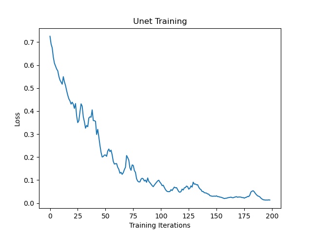
Run classification on test set
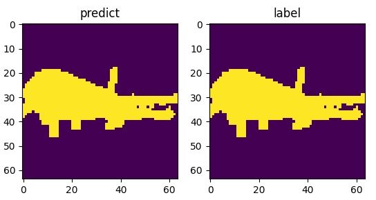
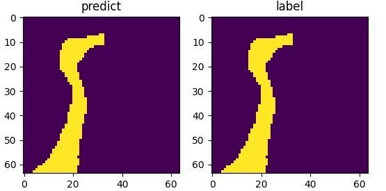
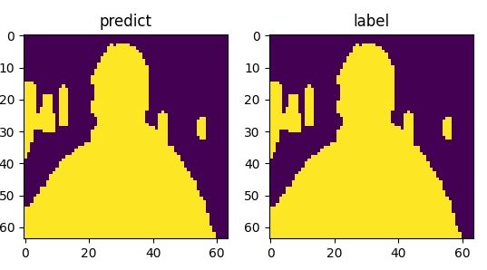
4.Hybrid quantum-classical QMLP network model
We introduce and analyze a proposed quantum multilayer perceptron (QMLP) architecture featuring fault-tolerant input embeddings, rich nonlinearities, and enhanced variational circuit simulations with parameterized two-qubit entanglement gates. QMLP: An Error-Tolerant Nonlinear Quantum MLP Architecture using Parameterized Two-Qubit Gates . We will write a simple example of integrating pyQPanda2 with VQNet.
Building Hybrid Classical-Quantum Neural Networks
import os
import gzip
import struct
import numpy as np
import pyqpanda as pq
from pyvqnet.nn.module import Module
from pyvqnet.nn.loss import MeanSquaredError, CrossEntropyLoss
from pyvqnet.optim.adam import Adam
from pyvqnet.tensor.tensor import QTensor
from pyvqnet.qnn.measure import expval
from pyvqnet.qnn.quantumlayer import QuantumLayer
from pyvqnet.nn.pooling import AvgPool2D
from pyvqnet.nn.linear import Linear
from pyvqnet.data.data import data_generator
from pyvqnet.tensor import tensor
import matplotlib
from matplotlib import pyplot as plt
try:
    matplotlib.use("TkAgg")
except:  # pylint:disable=bare-except
    print("Can not use matplot TkAgg")

try:
    import urllib.request
except ImportError:
    raise ImportError("You should use Python 3.x")

url_base = "https://ossci-datasets.s3.amazonaws.com/mnist/"
key_file = {
    "train_img": "train-images-idx3-ubyte.gz",
    "train_label": "train-labels-idx1-ubyte.gz",
    "test_img": "t10k-images-idx3-ubyte.gz",
    "test_label": "t10k-labels-idx1-ubyte.gz"
}


def _download(dataset_dir, file_name):
    """
    Download mnist data if needed.
    """
    file_path = dataset_dir + "/" + file_name

    if os.path.exists(file_path):
        with gzip.GzipFile(file_path) as file:
            file_path_ungz = file_path[:-3].replace("\\", "/")
            if not os.path.exists(file_path_ungz):
                open(file_path_ungz, "wb").write(file.read())
        return

    print("Downloading " + file_name + " ... ")
    urllib.request.urlretrieve(url_base + file_name, file_path)
    if os.path.exists(file_path):
        with gzip.GzipFile(file_path) as file:
            file_path_ungz = file_path[:-3].replace("\\", "/")
            file_path_ungz = file_path_ungz.replace("-idx", ".idx")
            if not os.path.exists(file_path_ungz):
                open(file_path_ungz, "wb").write(file.read())
    print("Done")

def download_mnist(dataset_dir):
    for v in key_file.values():
        _download(dataset_dir, v)

def load_mnist(dataset="training_data", digits=np.arange(2), path="./"):
    """
    load mnist data
    """
    from array import array as pyarray
    download_mnist(path)
    if dataset == "training_data":
        fname_image = os.path.join(path, "train-images.idx3-ubyte").replace(
            "\\", "/")
        fname_label = os.path.join(path, "train-labels.idx1-ubyte").replace(
            "\\", "/")
    elif dataset == "testing_data":
        fname_image = os.path.join(path, "t10k-images.idx3-ubyte").replace(
            "\\", "/")
        fname_label = os.path.join(path, "t10k-labels.idx1-ubyte").replace(
            "\\", "/")
    else:
        raise ValueError("dataset must be 'training_data' or 'testing_data'")

    flbl = open(fname_label, "rb")
    _, size = struct.unpack(">II", flbl.read(8))
    lbl = pyarray("b", flbl.read())
    flbl.close()

    fimg = open(fname_image, "rb")
    _, size, rows, cols = struct.unpack(">IIII", fimg.read(16))
    img = pyarray("B", fimg.read())
    fimg.close()

    ind = [k for k in range(size) if lbl[k] in digits]
    num = len(ind)
    images = np.zeros((num, rows, cols))
    labels = np.zeros((num, 1), dtype=int)
    for i in range(len(ind)):
        images[i] = np.array(img[ind[i] * rows * cols:(ind[i] + 1) * rows *
                                 cols]).reshape((rows, cols))
        labels[i] = lbl[ind[i]]

    return images, labels

def data_select(train_num, test_num):
    """
    Select data from mnist dataset.
    """
    x_train, y_train = load_mnist("training_data")
    x_test, y_test = load_mnist("testing_data")
    idx_train = np.append(
        np.where(y_train == 0)[0][:train_num],
        np.where(y_train == 1)[0][:train_num])

    x_train = x_train[idx_train]
    y_train = y_train[idx_train]

    x_train = x_train / 255
    y_train = np.eye(2)[y_train].reshape(-1, 2)

    # Test Leaving only labels 0 and 1
    idx_test = np.append(
        np.where(y_test == 0)[0][:test_num],
        np.where(y_test == 1)[0][:test_num])

    x_test = x_test[idx_test]
    y_test = y_test[idx_test]
    x_test = x_test / 255
    y_test = np.eye(2)[y_test].reshape(-1, 2)

    return x_train, y_train, x_test, y_test

def RotCircuit(para, qlist):

    if isinstance(para, QTensor):
        para = QTensor._to_numpy(para)
    if para.ndim > 1:
        raise ValueError(" dim of paramters in Rot should be 1")
    if para.shape[0] != 3:
        raise ValueError(" numbers of paramters in Rot should be 3")

    cir = pq.QCircuit()
    cir.insert(pq.RZ(qlist, para[2]))
    cir.insert(pq.RY(qlist, para[1]))
    cir.insert(pq.RZ(qlist, para[0]))

    return cir

def build_RotCircuit(qubits, weights):
    cir = pq.QCircuit()
    cir.insert(RotCircuit(weights[0:3], qubits[0]))
    cir.insert(RotCircuit(weights[3:6], qubits[1]))
    cir.insert(RotCircuit(weights[6:9], qubits[2]))
    cir.insert(RotCircuit(weights[9:12], qubits[3]))
    cir.insert(RotCircuit(weights[12:15], qubits[4]))
    cir.insert(RotCircuit(weights[15:18], qubits[5]))
    cir.insert(RotCircuit(weights[18:21], qubits[6]))
    cir.insert(RotCircuit(weights[21:24], qubits[7]))
    cir.insert(RotCircuit(weights[24:27], qubits[8]))
    cir.insert(RotCircuit(weights[27:30], qubits[9]))
    cir.insert(RotCircuit(weights[30:33], qubits[10]))
    cir.insert(RotCircuit(weights[33:36], qubits[11]))
    cir.insert(RotCircuit(weights[36:39], qubits[12]))
    cir.insert(RotCircuit(weights[39:42], qubits[13]))
    cir.insert(RotCircuit(weights[42:45], qubits[14]))
    cir.insert(RotCircuit(weights[45:48], qubits[15]))

    return cir

def CRXCircuit(para, control_qlists, rot_qlists):
    cir = pq.QCircuit()
    cir.insert(pq.RX(rot_qlists, para))
    cir.set_control(control_qlists)
    return cir

def build_CRotCircuit(qubits, weights):
    cir = pq.QCircuit()
    cir.insert(CRXCircuit(weights[0], qubits[0], qubits[1]))
    cir.insert(CRXCircuit(weights[1], qubits[1], qubits[2]))
    cir.insert(CRXCircuit(weights[2], qubits[2], qubits[3]))
    cir.insert(CRXCircuit(weights[3], qubits[3], qubits[4]))
    cir.insert(CRXCircuit(weights[4], qubits[4], qubits[5]))
    cir.insert(CRXCircuit(weights[5], qubits[5], qubits[6]))
    cir.insert(CRXCircuit(weights[6], qubits[6], qubits[7]))
    cir.insert(CRXCircuit(weights[7], qubits[7], qubits[8]))
    cir.insert(CRXCircuit(weights[8], qubits[8], qubits[9]))
    cir.insert(CRXCircuit(weights[9], qubits[9], qubits[10]))
    cir.insert(CRXCircuit(weights[10], qubits[10], qubits[11]))
    cir.insert(CRXCircuit(weights[11], qubits[11], qubits[12]))
    cir.insert(CRXCircuit(weights[12], qubits[12], qubits[13]))
    cir.insert(CRXCircuit(weights[13], qubits[13], qubits[14]))
    cir.insert(CRXCircuit(weights[14], qubits[14], qubits[15]))
    cir.insert(CRXCircuit(weights[15], qubits[15], qubits[0]))

    return cir


def build_qmlp_circuit(x, weights, qubits, clist, machine):
    cir = pq.QCircuit()
    num_qubits = len(qubits)
    for i in range(num_qubits):
        cir.insert(pq.RX(qubits[i], x[i]))

    cir.insert(build_RotCircuit(qubits, weights[0:48]))
    cir.insert(build_CRotCircuit(qubits, weights[48:64]))

    for i in range(num_qubits):
        cir.insert(pq.RX(qubits[i], x[i]))

    cir.insert(build_RotCircuit(qubits, weights[64:112]))
    cir.insert(build_CRotCircuit(qubits, weights[112:128]))

    prog = pq.QProg()
    prog.insert(cir)
    # print(prog)
    # exit()

    exp_vals = []
    for position in range(num_qubits):
        pauli_str = {"Z" + str(position): 1.0}
        exp2 = expval(machine, prog, pauli_str, qubits)
        exp_vals.append(exp2)

    return exp_vals


class QMLPModel(Module):
    def __init__(self):
        super(QMLPModel, self).__init__()
        self.ave_pool2d = AvgPool2D([7, 7], [7, 7], "valid")
        self.quantum_circuit = QuantumLayer(build_qmlp_circuit, 128, "CPU", 16, diff_method="finite_diff")

        self.linear = Linear(16, 10)

    def forward(self, x):
        bsz = x.shape[0]
        x = self.ave_pool2d(x)
        input_data = x.reshape([bsz, 16])
        quanutum_result = self.quantum_circuit(input_data)
        result = self.linear(quanutum_result)
        return result

def vqnet_test_QMLPModel():
    # train num=1000, test_num=100
    # x_train, y_train, x_test, y_test = data_select(1000, 100)

    train_size = 1000
    eval_size = 100
    x_train, y_train = load_mnist("training_data", digits=np.arange(10))
    x_test, y_test = load_mnist("testing_data", digits=np.arange(10))

    x_train = x_train[:train_size]
    y_train = y_train[:train_size]
    x_test = x_test[:eval_size]
    y_test = y_test[:eval_size]

    x_train = x_train / 255
    x_test = x_test / 255
    y_train = np.eye(10)[y_train].reshape(-1, 10)
    y_test = np.eye(10)[y_test].reshape(-1, 10)

    model = QMLPModel()
    optimizer = Adam(model.parameters(), lr=0.005)
    loss_func = CrossEntropyLoss()
    loss_list = []
    epochs = 30
    for epoch in range(1, epochs):
        total_loss = []

        correct = 0
        n_train = 0
        for x, y in data_generator(x_train,
                                   y_train,
                                   batch_size=16,
                                   shuffle=True):

            x = x.reshape(-1, 1, 28, 28)
            optimizer.zero_grad()
            # Forward pass
            output = model(x)
            # Calculating loss
            loss = loss_func(y, output)
            loss_np = np.array(loss.data)
            print("loss: ", loss_np)
            np_output = np.array(output.data, copy=False)

            temp_out = np_output.argmax(axis=1)
            temp_output = np.zeros((temp_out.size, 10))
            temp_output[np.arange(temp_out.size), temp_out] = 1
            temp_maks = (temp_output == y)

            correct += np.sum(np.array(temp_maks))
            n_train += 160

            # Backward pass
            loss.backward()
            # Optimize the weights
            optimizer._step()
            total_loss.append(loss_np)
        print("##########################")
        print(f"Train Accuracy: {correct / n_train}")
        loss_list.append(np.sum(total_loss) / len(total_loss))
        # train_acc_list.append(correct / n_train)
        print("epoch: ", epoch)
        # print(100. * (epoch + 1) / epochs)
        print("{:.0f} loss is : {:.10f}".format(epoch, loss_list[-1]))

if __name__ == "__main__":

    vqnet_test_QMLPModel()
data result
The loss function curve of the training data is displayed and saved, and the results of the test data are saved. Loss situation on the training set.
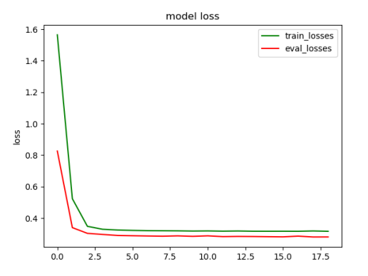
5.Hybrid quantum-classical QDRL network model
We introduce and analyze a proposed quantum reinforcement learning network (QDRL), whose features reshape classical deep reinforcement learning algorithms such as experience replay and target networks into representations of variational quantum circuits. Furthermore, we use a quantum information encoding scheme to reduce the number of model parameters compared to classical neural networks. QDRL: Variational Quantum Circuits for Deep Reinforcement Learning. We will write a simple example of integrating pyQPanda2 with VQNet.
Building Hybrid Classical-Quantum Neural Networks
Requires gym == 0.23.0 , pygame == 2.1.2 .
import numpy as np
import random
import gym
import time
from matplotlib import animation
import pyqpanda as pq
from pyvqnet.nn.module import Module
from pyvqnet.nn.loss import MeanSquaredError
from pyvqnet.optim.adam import Adam
from pyvqnet.tensor.tensor import QTensor
from pyvqnet import kfloat32
from pyvqnet.qnn.quantumlayer import QuantumLayer
from pyvqnet.tensor import tensor
from pyvqnet.qnn.measure import expval
from pyvqnet._core import Tensor as CoreTensor
import matplotlib
from matplotlib import pyplot as plt
try:
    matplotlib.use("TkAgg")
except:  # pylint:disable=bare-except
    print("Can not use matplot TkAgg")
def display_frames_as_gif(frames, c_index):
    patch = plt.imshow(frames[0])
    plt.axis('off')
    def animate(i):
        patch.set_data(frames[i])
    anim = animation.FuncAnimation(plt.gcf(), animate, frames=len(frames), interval=5)
    name_result = "./result_"+str(c_index)+".gif"
    anim.save(name_result, writer='pillow', fps=10)
CIRCUIT_SIZE = 4
MAX_ITERATIONS = 50
MAX_STEPS = 250
BATCHSIZE = 5
TARGET_MAX = 20
GAMMA = 0.99
STATE_T = 0
ACTION = 1
REWARD = 2
STATE_NT = 3
DONE = 4
def RotCircuit(para, qlist):

    if isinstance(para, QTensor):
        para = QTensor._to_numpy(para)
    if para.ndim > 1:
        raise ValueError(" dim of paramters in Rot should be 1")
    if para.shape[0] != 3:
        raise ValueError(" numbers of paramters in Rot should be 3")
    cir = pq.QCircuit()
    cir.insert(pq.RZ(qlist, para[2]))
    cir.insert(pq.RY(qlist, para[1]))
    cir.insert(pq.RZ(qlist, para[0]))
    return cir
def layer_circuit(qubits, weights):
    cir = pq.QCircuit()
    # Entanglement block
    cir.insert(pq.CNOT(qubits[0], qubits[1]))
    cir.insert(pq.CNOT(qubits[1], qubits[2]))
    cir.insert(pq.CNOT(qubits[2], qubits[3]))
    # u3 gate
    cir.insert(RotCircuit(weights[0], qubits[0]))  # weights shape = [4, 3]
    cir.insert(RotCircuit(weights[1], qubits[1]))
    cir.insert(RotCircuit(weights[2], qubits[2]))
    cir.insert(RotCircuit(weights[3], qubits[3]))
    return cir
def encoder(encodings):
    encodings = int(encodings[0])
    return [i for i, b in enumerate(f'{encodings:0{CIRCUIT_SIZE}b}') if b == '1']

def build_qc(x, weights, qubits, cubits ,machine):


    cir = pq.QCircuit()
    if x:
        wires = encoder(x)
        for wire in wires:
            cir.insert(pq.RX(qubits[wire], np.pi))
            cir.insert(pq.RZ(qubits[wire], np.pi))
    # parameter number = 24
    weights = weights.reshape([2, 4, 3])
    # layer wise
    for w in weights:
        cir.insert(layer_circuit(qubits, w))
    prog = pq.QProg()
    prog.insert(cir)
    exp_vals = []
    for position in range(n_qubits):
        pauli_str = {"Z" + str(position): 1.0}
        exp2 = expval(machine, prog, pauli_str, qubits)
        exp_vals.append(exp2)
    return exp_vals
class DRLModel(Module):
    def __init__(self):
        super(DRLModel, self).__init__()
        self.quantum_circuit = QuantumLayer(build_qc, 24, "CPU", 4, diff_method="finite_diff")

    def forward(self, x):
        quanutum_result = self.quantum_circuit(x)
        return quanutum_result
env = gym.make("FrozenLake-v1", is_slippery = False, map_name = '4x4')
state = env.reset()
n_layers = 2
n_qubits = 4
targ_counter = 0
sampled_vs = []
memory = {}
param = QTensor(0.01 * np.random.randn(n_layers, n_qubits, 3))
bias = QTensor([[0.0, 0.0, 0.0, 0.0]])
param_targ = param.copy().reshape([1, -1]).pdata[0]
bias_targ = bias.copy()
loss_func = MeanSquaredError()
model = DRLModel()
opt = Adam(model.parameters(), lr=5)
for i in range(MAX_ITERATIONS):
    start = time.time()
    state_t = env.reset()
    a_init = env.action_space.sample()
    total_reward = 0
    done = False
    frames = []
    for t in range(MAX_STEPS):
        frames.append(env.render(mode='rgb_array'))
        time.sleep(0.1)
        input_x = QTensor([[state_t]],dtype=kfloat32)
        acts = model(input_x) + bias

        act_t = tensor.QTensor.argmax(acts)

        act_t_np = int(act_t.pdata[0])
        print(f'Episode: {i}, Steps: {t}, act: {act_t_np}')
        state_nt, reward, done, info = env.step(action=act_t_np)
        targ_counter += 1
        input_state_nt = QTensor([[state_nt]],dtype=kfloat32)
        act_nt = QTensor.argmax(model(input_state_nt)+bias)
        act_nt_np = int(act_nt.pdata[0])
        memory[i, t] = (state_t, act_t, reward, state_nt, done)
        if len(memory) >= BATCHSIZE:
            # print('Optimizing...')
            sampled_vs = [memory[k] for k in random.sample(list(memory), BATCHSIZE)]
            target_temp = []
            for s in sampled_vs:
                if s[DONE]:
                    target_temp.append(QTensor(s[REWARD]).reshape([1, -1]))
                else:
                    input_s = QTensor([[s[STATE_NT]]],dtype=kfloat32)
                    out_temp = s[REWARD] + GAMMA * tensor.max(model(input_s) + bias_targ)
                    out_temp = out_temp.reshape([1, -1])
                    target_temp.append(out_temp)
            target_out = []
            for b in sampled_vs:
                input_b = QTensor([[b[STATE_T]]], requires_grad=True,dtype=kfloat32)
                out_result = model(input_b) + bias
                index = int(b[ACTION].pdata[0])
                out_result_temp = out_result[0][index].reshape([1, -1])
                target_out.append(out_result_temp)
            opt.zero_grad()
            target_label = tensor.concatenate(target_temp, 1)
            output = tensor.concatenate(target_out, 1)
            loss = loss_func(target_label, output)
            loss.backward()
            opt.step()
        # update parameters in target circuit
        if targ_counter == TARGET_MAX:
            param_targ = param.copy().reshape([1, -1]).pdata[0]
            bias_targ = bias.copy()
            targ_counter = 0
        state_t, act_t_np = state_nt, act_nt_np
        if done:
            print("reward", reward)
            if reward == 1.0:
                frames.append(env.render(mode='rgb_array'))
                display_frames_as_gif(frames, i)
                exit()
            break
    end = time.time()
Unsupervised learning
1 Quantum Kmeans
1.1 Introduction
Clustering algorithm is a typical unsupervised learning algorithm, which is mainly used to automatically classify similar samples into one class. In the clustering algorithm, samples are divided into different categories according to the similarity between samples. For different similarity calculation methods, different clustering results will be obtained. The common similarity calculation method is Euclidean distance method. What we want to show is the quantum k-means algorithm. K-means algorithm is a distance based clustering algorithm. It takes distance as the evaluation index of similarity, that is, the closer the distance between two objects, the greater the similarity. The algorithm considers that clusters are composed of objects close to each other, so compact and independent clusters are the ultimate goal.
Quantum kmeans quantum machine learning model can also be developed in VQNet. An example of the quantum kmeans clustering task is given below. Through the quantum circuit, we can construct a measurement that is positively correlated with the Euclidean distance of the variables of classical machine learning, so as to achieve the goal of finding the nearest neighbor.
1.2 Introduction to algorithm principle
The implementation of quantum k-means algorithm mainly uses swap test to compare the distance between input data points. Randomly select k points from N data points as centroids, measure the distance from each point to each centroid, assign it to the nearest centroid class, recalculate the centroid of each class, and iterate 2 to 3 steps until the new centroid is equal to or less than the specified threshold. In our example, we select 100 data points and 2 centroids, and use cswap circuit to calculate the distance. Finally, we obtained two data point clusters. \(|0\rangle\) is an auxiliary bit, through the H logic gate, the qubit will become \(\frac{1}{\sqrt{2}}(|0\rangle + |1\rangle)\). Under the control of \(|1\rangle\) qubit, The quantum circuit will flip \(|x\rangle\) and \(|y\rangle\) . Finally get the result:
If we measure the auxiliary qubit separately, the probability of the final state of the ground state \(|1\rangle\) is:
The Euclidean distance between two quantum states is as follows:
Visible measurement qubit \(|1\rangle\) is positively correlated with Euclidean distance. The quantum circuit of this algorithm is as follows:
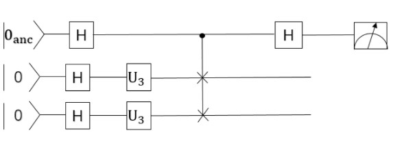
1.3 VQNet implementation
1.3.1 Environmental preparation
The environment adopts Python 3 8. It is recommended to use CONDA for environment configuration. It comes with numpy, SciPy, Matplotlib, sklearn and other toolkits for easy use. If the python environment is adopted, relevant packages need to be installed, and the following environment pyvqnet needs to be prepared
1.3.2 Data preparation
The data is randomly generated by make_blobs under SciPy, and the function is defined to generate Gaussian distribution data.
import sys
sys.path.insert(0, "../")
import math
import numpy as np
from pyvqnet.tensor.tensor import QTensor, zeros
import pyvqnet.tensor.tensor as tensor
import pyqpanda as pq
from sklearn.datasets import make_blobs
import matplotlib.pyplot as plt
import matplotlib
try:
    matplotlib.use("TkAgg")
except:
    print("Can not use matplot TkAgg")
    pass

def get_data(n, k, std):
    data = make_blobs(n_samples=n,
                    n_features=2,
                    centers=k,
                    cluster_std=std,
                    random_state=100)
    points = data[0]
    centers = data[1]
    return points, centers
1.3.3 Quantum circuit
Constructing quantum circuits using VQNet
# The input quantum gate rotation angle is calculated according to the input coordinate point d (x, y)
def get_theta(d):
    x = d[0]
    y = d[1]
    theta = 2 * math.acos((x.item() + y.item()) / 2.0)
    return theta

# The quantum circuit is constructed according to the input quantum data points
def qkmeans_circuits(x, y):

    theta_1 = get_theta(x)
    theta_2 = get_theta(y)

    num_qubits = 3
    machine = pq.CPUQVM()
    machine.init_qvm()
    qubits = machine.qAlloc_many(num_qubits)
    cbits = machine.cAlloc_many(num_qubits)
    circuit = pq.QCircuit()

    circuit.insert(pq.H(qubits[0]))
    circuit.insert(pq.H(qubits[1]))
    circuit.insert(pq.H(qubits[2]))

    circuit.insert(pq.U3(qubits[1], theta_1, np.pi, np.pi))
    circuit.insert(pq.U3(qubits[2], theta_2, np.pi, np.pi))

    circuit.insert(pq.SWAP(qubits[1], qubits[2]).control([qubits[0]]))

    circuit.insert(pq.H(qubits[0]))

    prog = pq.QProg()
    prog.insert(circuit)
    prog << pq.Measure(qubits[0], cbits[0])
    prog.insert(pq.Reset(qubits[0]))
    prog.insert(pq.Reset(qubits[1]))
    prog.insert(pq.Reset(qubits[2]))

    result = machine.run_with_configuration(prog, cbits, 1024)

    data = result

    if len(data) == 1:
        return 0.0
    else:
        return data['001'] / 1024.0
1.3.4 Data visualization
Visual calculation of relevant clustering data
# Visualization of scatter points and cluster centers
def draw_plot(points, centers, label=True):
    points = np.array(points)
    centers = np.array(centers)
    if label==False:
        plt.scatter(points[:,0], points[:,1])
    else:
        plt.scatter(points[:,0], points[:,1], c=centers, cmap='viridis')
    plt.xlim(0, 1)
    plt.ylim(0, 1)
    plt.show()
1.3.5 Cluster calculation
Calculate the cluster center of relevant cluster data
# Randomly generate cluster center points
def initialize_centers(points,k):
    return points[np.random.randint(points.shape[0],size=k),:]


def find_nearest_neighbour(points, centroids):
    n = points.shape[0]
    k = centroids.shape[0]

    centers = zeros([n], dtype=points.dtype)

    for i in range(n):
        min_dis = 10000
        ind = 0
        for j in range(k):

            temp_dis = qkmeans_circuits(points[i, :], centroids[j, :])

            if temp_dis < min_dis:
                min_dis = temp_dis
                ind = j
        centers[i] = ind

    return centers

def find_centroids(points, centers):

    k = int(tensor.max(centers).item()) + 1
    centroids = tensor.zeros([k, 2], dtype=points.dtype)
    for i in range(k):

        cur_i = centers == i

        x = points[:,0]
        x = x[cur_i]
        y = points[:,1]
        y = y[cur_i]
        centroids[i, 0] = tensor.mean(x)
        centroids[i, 1] = tensor.mean(y)

    return centroids

def preprocess(points):
    n = len(points)
    x = 30.0 * np.sqrt(2)
    for i in range(n):
        points[i, :] += 15
        points[i, :] /= x

    return points


def qkmean_run():
    n = 100  # number of data points
    k = 3  # Number of centers
    std = 2  # std of datapoints

    points, o_centers = get_data(n, k, std)  # dataset

    points = preprocess(points)  # Normalize dataset

    centroids = initialize_centers(points, k)  # Intialize centroids

    epoch = 9
    points = QTensor(points)
    centroids = QTensor(centroids)
    plt.figure()
    draw_plot(points.data, o_centers,label=False)

    for i in range(epoch):
            centers = find_nearest_neighbour(points, centroids)  # find nearest centers
            centroids = find_centroids(points, centers)  # find centroids

    plt.figure()
    draw_plot(points.data, centers.data)

# Run program entry
if __name__ == "__main__":
    qkmean_run()
1.3.6 Data distribution before clustering
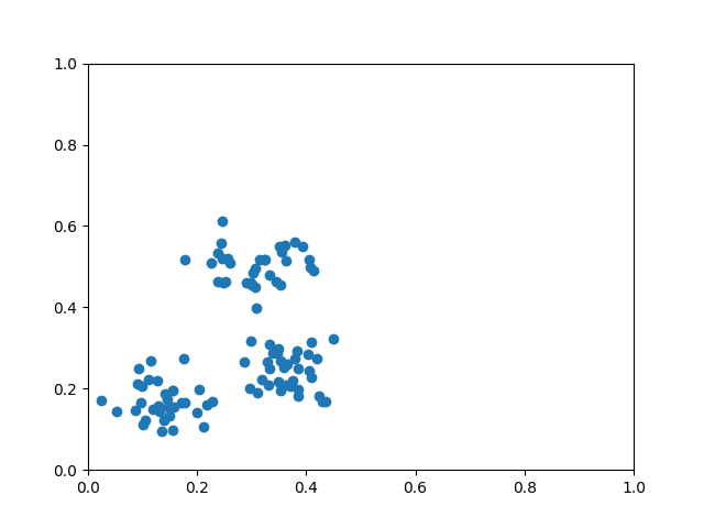
1.3.7 Data distribution after clustering
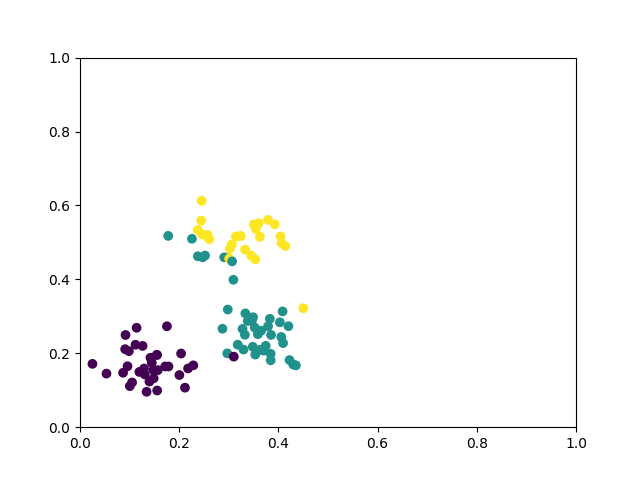
Quantum Machine Learning Research
Quantum models as Fourier series
Quantum computers can be used for supervised learning by treating parametrised quantum circuits as models that map data inputs to predictions. While a lot of work has been done to investigate practical implications of this approach, many important theoretical properties of these models remain unknown. Here we investigate how the strategy with which data is encoded into the model influences the expressive power of parametrised quantum circuits as function approximators.
The paper The effect of data encoding on the expressive power of variational quantum machine learning models links common quantum machine learning models designed for near-term quantum computers to Fourier series
1.1Fitting Fourier series with serial Pauli-rotation encoding
First we show how quantum models that use Pauli rotations as data-encoding gates can only fit Fourier series up to a certain degree. For simplicity we will only look at single-qubit circuits:
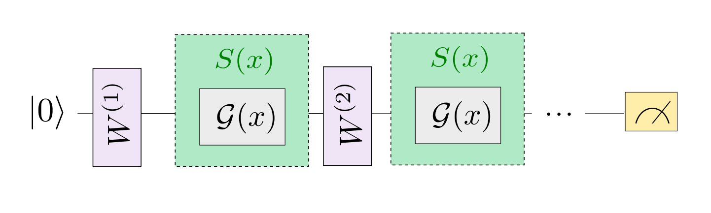
Make input data, define parallel quantum models, and do not perform model training results.
"""
Quantum Fourier Series
"""
import numpy as np
import pyqpanda as pq
from pyvqnet.qnn.measure import expval
import matplotlib.pyplot as plt
import matplotlib
try:
    matplotlib.use("TkAgg")
except:  # pylint:disable=bare-except
    print("Can not use matplot TkAgg")
    pass

np.random.seed(42)


degree = 1  # degree of the target function
scaling = 1  # scaling of the data
coeffs = [0.15 + 0.15j]*degree  # coefficients of non-zero frequencies
coeff0 = 0.1  # coefficient of zero frequency

def target_function(x):
    """Generate a truncated Fourier series, where the data gets re-scaled."""
    res = coeff0
    for idx, coeff in enumerate(coeffs):
        exponent = np.complex128(scaling * (idx+1) * x * 1j)
        conj_coeff = np.conjugate(coeff)
        res += coeff * np.exp(exponent) + conj_coeff * np.exp(-exponent)
    return np.real(res)

x = np.linspace(-6, 6, 70)
target_y = np.array([target_function(x_) for x_ in x])

plt.plot(x, target_y, c='black')
plt.scatter(x, target_y, facecolor='white', edgecolor='black')
plt.ylim(-1, 1)
plt.show()


def S(scaling, x, qubits):
    cir = pq.QCircuit()
    cir.insert(pq.RX(qubits[0], scaling * x))
    return cir

def W(theta, qubits):
    cir = pq.QCircuit()
    cir.insert(pq.RZ(qubits[0], theta[0]))
    cir.insert(pq.RY(qubits[0], theta[1]))
    cir.insert(pq.RZ(qubits[0], theta[2]))
    return cir

def serial_quantum_model(weights, x, num_qubits, scaling):
    cir = pq.QCircuit()
    machine = pq.CPUQVM()  # outside
    machine.init_qvm()  # outside
    qubits = machine.qAlloc_many(num_qubits)

    for theta in weights[:-1]:
        cir.insert(W(theta, qubits))
        cir.insert(S(scaling, x, qubits))

    # (L+1)'th unitary
    cir.insert(W(weights[-1], qubits))
    prog = pq.QProg()
    prog.insert(cir)

    exp_vals = []
    for position in range(num_qubits):
        pauli_str = {"Z" + str(position): 1.0}
        exp2 = expval(machine, prog, pauli_str, qubits)
        exp_vals.append(exp2)

    return exp_vals

r = 1
weights = 2 * np.pi * np.random.random(size=(r+1, 3))  # some random initial weights

x = np.linspace(-6, 6, 70)
random_quantum_model_y = [serial_quantum_model(weights, x_, 1, 1) for x_ in x]

plt.plot(x, target_y, c='black', label="true")
plt.scatter(x, target_y, facecolor='white', edgecolor='black')
plt.plot(x, random_quantum_model_y, c='blue', label="predict")
plt.ylim(-1, 1)
plt.legend(loc="upper right")
plt.show()
The result of running the quantum circuit without training is:
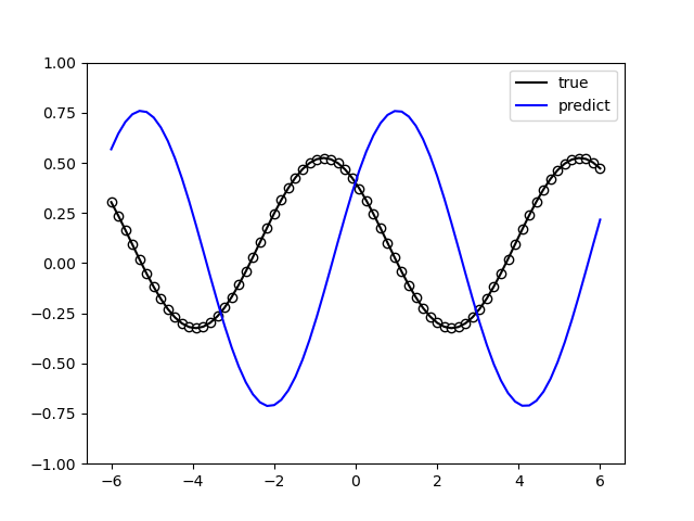
Make the input data, define the serial quantum model, and build the training model in combination with the QuantumLayer of the VQNet framework.
"""
Quantum Fourier Series Serial
"""
import numpy as np
from pyvqnet.nn.module import Module
from pyvqnet.nn.loss import MeanSquaredError
from pyvqnet.optim.adam import Adam
from pyvqnet.tensor.tensor import QTensor
import pyqpanda as pq
from pyvqnet.qnn.measure import expval
from pyvqnet.qnn.quantumlayer import QuantumLayer
import matplotlib.pyplot as plt
import matplotlib
try:
    matplotlib.use("TkAgg")
except:  # pylint:disable=bare-except
    print("Can not use matplot TkAgg")
    pass

np.random.seed(42)

degree = 1  # degree of the target function
scaling = 1  # scaling of the data
coeffs = [0.15 + 0.15j]*degree  # coefficients of non-zero frequencies
coeff0 = 0.1  # coefficient of zero frequency

def target_function(x):
    """Generate a truncated Fourier series, where the data gets re-scaled."""
    res = coeff0
    for idx, coeff in enumerate(coeffs):
        exponent = np.complex128(scaling * (idx+1) * x * 1j)
        conj_coeff = np.conjugate(coeff)
        res += coeff * np.exp(exponent) + conj_coeff * np.exp(-exponent)
    return np.real(res)

x = np.linspace(-6, 6, 70)
target_y = np.array([target_function(xx) for xx in x])

plt.plot(x, target_y, c='black')
plt.scatter(x, target_y, facecolor='white', edgecolor='black')
plt.ylim(-1, 1)
plt.show()


def S(x, qubits):
    cir = pq.QCircuit()
    cir.insert(pq.RX(qubits[0], x))
    return cir

def W(theta, qubits):
    cir = pq.QCircuit()
    cir.insert(pq.RZ(qubits[0], theta[0]))
    cir.insert(pq.RY(qubits[0], theta[1]))
    cir.insert(pq.RZ(qubits[0], theta[2]))
    return cir


r = 1
weights = 2 * np.pi * np.random.random(size=(r+1, 3))  # some random initial weights

x = np.linspace(-6, 6, 70)


def q_circuits_loop(x, weights, qubits, clist, machine):

    result = []
    for xx in x:
        cir = pq.QCircuit()
        weights = weights.reshape([2, 3])

        for theta in weights[:-1]:
            cir.insert(W(theta, qubits))
            cir.insert(S(xx, qubits))

        cir.insert(W(weights[-1], qubits))
        prog = pq.QProg()
        prog.insert(cir)

        exp_vals = []
        for position in range(1):
            pauli_str = {"Z" + str(position): 1.0}
            exp2 = expval(machine, prog, pauli_str, qubits)
            exp_vals.append(exp2)
            result.append(exp2)
    return result

class Model(Module):
    def __init__(self):
        super(Model, self).__init__()
        self.q_fourier_series = QuantumLayer(q_circuits_loop, 6, "CPU", 1)

    def forward(self, x):
        return self.q_fourier_series(x)

def run():
    model = Model()

    optimizer = Adam(model.parameters(), lr=0.5)
    batch_size = 2
    epoch = 5
    loss = MeanSquaredError()
    print("start training..............")
    model.train()
    max_steps = 50
    for i in range(epoch):
        sum_loss = 0
        count = 0
        for step in range(max_steps):
            optimizer.zero_grad()
            # Select batch of data
            batch_index = np.random.randint(0, len(x), (batch_size,))
            x_batch = x[batch_index]
            y_batch = target_y[batch_index]
            data, label = QTensor([x_batch]), QTensor([y_batch])
            result = model(data)
            loss_b = loss(label, result)
            loss_b.backward()
            optimizer._step()
            sum_loss += loss_b.item()
            count += batch_size
        print(f"epoch:{i}, #### loss:{sum_loss/count} ")

        model.eval()
        predictions = []
        for xx in x:
            data = QTensor([[xx]])
            result = model(data)
            predictions.append(result.pdata[0])

        plt.plot(x, target_y, c='black', label="true")
        plt.scatter(x, target_y, facecolor='white', edgecolor='black')
        plt.plot(x, predictions, c='blue', label="predict")
        plt.ylim(-1, 1)
        plt.legend(loc="upper right")
        plt.show()

if __name__ == "__main__":
    run()
The quantum model is:

The network training results are:
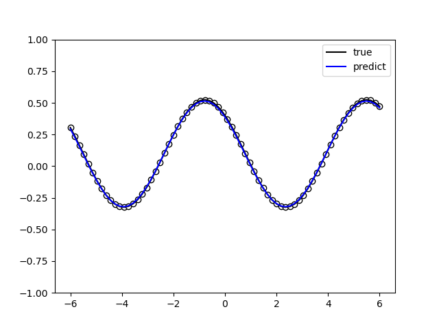
The network training loss is:
start training..............
epoch:0, #### loss:0.04852807720773853
epoch:1, #### loss:0.012945819365559146
epoch:2, #### loss:0.0009359727291666786
epoch:3, #### loss:0.00015995280153333625
epoch:4, #### loss:3.988249877352246e-05
1.2Fitting Fourier series with parallel Pauli-rotation encoding
As shown in the paper, we expect similar results to the serial model: a Fourier series of order r can only be fitted if the encoded gate has at least r repetitions in the quantum model. Quantum circuit:
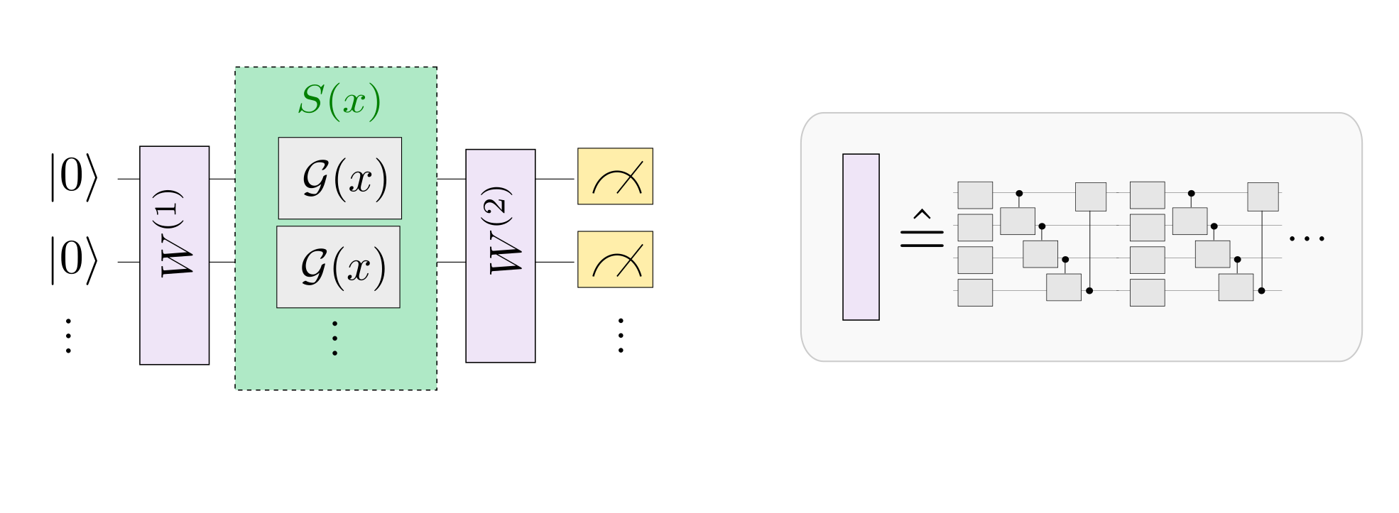
Make input data, define parallel quantum models, and do not perform model training results.
"""
Quantum Fourier Series
"""
import numpy as np
import pyqpanda as pq
from pyvqnet.qnn.measure import expval
import matplotlib.pyplot as plt
import matplotlib
try:
    matplotlib.use("TkAgg")
except:  # pylint:disable=bare-except
    print("Can not use matplot TkAgg")
    pass

np.random.seed(42)

degree = 1  # degree of the target function
scaling = 1  # scaling of the data
coeffs = [0.15 + 0.15j] * degree  # coefficients of non-zero frequencies
coeff0 = 0.1  # coefficient of zero frequency

def target_function(x):
    """Generate a truncated Fourier series, where the data gets re-scaled."""
    res = coeff0
    for idx, coeff in enumerate(coeffs):
        exponent = np.complex128(scaling * (idx + 1) * x * 1j)
        conj_coeff = np.conjugate(coeff)
        res += coeff * np.exp(exponent) + conj_coeff * np.exp(-exponent)
    return np.real(res)

x = np.linspace(-6, 6, 70)
target_y = np.array([target_function(xx) for xx in x])


def S1(x, qubits):
    cir = pq.QCircuit()
    for q in qubits:
        cir.insert(pq.RX(q, x))
    return cir

def W1(theta, qubits):
    cir = pq.QCircuit()
    for i in range(len(qubits)):
        cir.insert(pq.RZ(qubits[i], theta[0][i][0]))
        cir.insert(pq.RY(qubits[i], theta[0][i][1]))
        cir.insert(pq.RZ(qubits[i], theta[0][i][2]))

    for i in range(len(qubits) - 1):
        cir.insert(pq.CNOT(qubits[i], qubits[i + 1]))
    cir.insert(pq.CNOT(qubits[len(qubits) - 1], qubits[0]))

    for i in range(len(qubits)):
        cir.insert(pq.RZ(qubits[i], theta[1][i][0]))
        cir.insert(pq.RY(qubits[i], theta[1][i][1]))
        cir.insert(pq.RZ(qubits[i], theta[1][i][2]))

    cir.insert(pq.CNOT(qubits[0], qubits[len(qubits) - 1]))
    for i in range(len(qubits) - 1):
        cir.insert(pq.CNOT(qubits[i + 1], qubits[i]))

    for i in range(len(qubits)):
        cir.insert(pq.RZ(qubits[i], theta[2][i][0]))
        cir.insert(pq.RY(qubits[i], theta[2][i][1]))
        cir.insert(pq.RZ(qubits[i], theta[2][i][2]))

    for i in range(len(qubits) - 1):
        cir.insert(pq.CNOT(qubits[i], qubits[i + 1]))
    cir.insert(pq.CNOT(qubits[len(qubits) - 1], qubits[0]))

    return cir

def parallel_quantum_model(weights, x, num_qubits):
    cir = pq.QCircuit()
    machine = pq.CPUQVM()  # outside
    machine.init_qvm()  # outside
    qubits = machine.qAlloc_many(num_qubits)

    cir.insert(W1(weights[0], qubits))
    cir.insert(S1(x, qubits))

    cir.insert(W1(weights[1], qubits))
    prog = pq.QProg()
    prog.insert(cir)

    exp_vals = []
    for position in range(1):
        pauli_str = {"Z" + str(position): 1.0}
        exp2 = expval(machine, prog, pauli_str, qubits)
        exp_vals.append(exp2)

    return exp_vals

r = 3

trainable_block_layers = 3
weights = 2 * np.pi * np.random.random(size=(2, trainable_block_layers, r, 3))
# print(weights)
x = np.linspace(-6, 6, 70)
random_quantum_model_y = [parallel_quantum_model(weights, xx, r) for xx in x]

plt.plot(x, target_y, c='black', label="true")
plt.scatter(x, target_y, facecolor='white', edgecolor='black')
plt.plot(x, random_quantum_model_y, c='blue', label="predict")
plt.ylim(-1, 1)
plt.legend(loc="upper right")
plt.show()
The result of running the quantum circuit without training is:
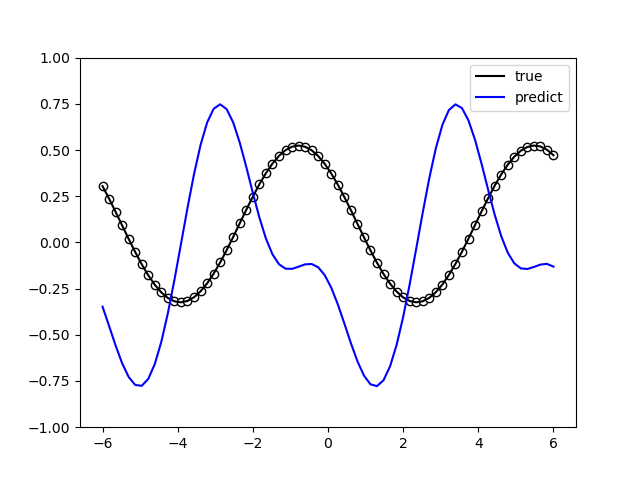
Make the input data, define the parallel quantum model, and build the training model in combination with the QuantumLayer layer of the VQNet framework.
"""
Quantum Fourier Series
"""
import numpy as np

from pyvqnet.nn.module import Module
from pyvqnet.nn.loss import MeanSquaredError
from pyvqnet.optim.adam import Adam
from pyvqnet.tensor.tensor import QTensor
import pyqpanda as pq
from pyvqnet.qnn.measure import expval
from pyvqnet.qnn.quantumlayer import QuantumLayer
import matplotlib.pyplot as plt
import matplotlib
try:
    matplotlib.use("TkAgg")
except:  # pylint:disable=bare-except
    print("Can not use matplot TkAgg")
    pass

np.random.seed(42)

degree = 1  # degree of the target function
scaling = 1  # scaling of the data
coeffs = [0.15 + 0.15j] * degree  # coefficients of non-zero frequencies
coeff0 = 0.1  # coefficient of zero frequency

def target_function(x):
    """Generate a truncated Fourier series, where the data gets re-scaled."""
    res = coeff0
    for idx, coeff in enumerate(coeffs):
        exponent = np.complex128(scaling * (idx + 1) * x * 1j)
        conj_coeff = np.conjugate(coeff)
        res += coeff * np.exp(exponent) + conj_coeff * np.exp(-exponent)
    return np.real(res)

x = np.linspace(-6, 6, 70)
target_y = np.array([target_function(xx) for xx in x])

plt.plot(x, target_y, c='black')
plt.scatter(x, target_y, facecolor='white', edgecolor='black')
plt.ylim(-1, 1)
plt.show()

def S1(x, qubits):
    cir = pq.QCircuit()
    for q in qubits:
        cir.insert(pq.RX(q, x))
    return cir

def W1(theta, qubits):
    cir = pq.QCircuit()
    for i in range(len(qubits)):
        cir.insert(pq.RZ(qubits[i], theta[0][i][0]))
        cir.insert(pq.RY(qubits[i], theta[0][i][1]))
        cir.insert(pq.RZ(qubits[i], theta[0][i][2]))

    for i in range(len(qubits) - 1):
        cir.insert(pq.CNOT(qubits[i], qubits[i + 1]))
    cir.insert(pq.CNOT(qubits[len(qubits) - 1], qubits[0]))

    for i in range(len(qubits)):
        cir.insert(pq.RZ(qubits[i], theta[1][i][0]))
        cir.insert(pq.RY(qubits[i], theta[1][i][1]))
        cir.insert(pq.RZ(qubits[i], theta[1][i][2]))

    cir.insert(pq.CNOT(qubits[0], qubits[len(qubits) - 1]))
    for i in range(len(qubits) - 1):
        cir.insert(pq.CNOT(qubits[i + 1], qubits[i]))

    for i in range(len(qubits)):
        cir.insert(pq.RZ(qubits[i], theta[2][i][0]))
        cir.insert(pq.RY(qubits[i], theta[2][i][1]))
        cir.insert(pq.RZ(qubits[i], theta[2][i][2]))

    for i in range(len(qubits) - 1):
        cir.insert(pq.CNOT(qubits[i], qubits[i + 1]))
    cir.insert(pq.CNOT(qubits[len(qubits) - 1], qubits[0]))

    return cir

def q_circuits_loop(x, weights, qubits, clist, machine):

    result = []
    for xx in x:
        cir = pq.QCircuit()
        weights = weights.reshape([2, 3, 3, 3])

        cir.insert(W1(weights[0], qubits))
        cir.insert(S1(xx, qubits))

        cir.insert(W1(weights[1], qubits))
        prog = pq.QProg()
        prog.insert(cir)

        exp_vals = []
        for position in range(1):
            pauli_str = {"Z" + str(position): 1.0}
            exp2 = expval(machine, prog, pauli_str, qubits)
            exp_vals.append(exp2)
            result.append(exp2)
    return result


class Model(Module):
    def __init__(self):
        super(Model, self).__init__()

        self.q_fourier_series = QuantumLayer(q_circuits_loop, 2 * 3 * 3 * 3, "CPU", 3)

    def forward(self, x):
        return self.q_fourier_series(x)

def run():
    model = Model()

    optimizer = Adam(model.parameters(), lr=0.01)
    batch_size = 2
    epoch = 5
    loss = MeanSquaredError()
    print("start training..............")
    model.train()
    max_steps = 50
    for i in range(epoch):
        sum_loss = 0
        count = 0
        for step in range(max_steps):
            optimizer.zero_grad()
            # Select batch of data
            batch_index = np.random.randint(0, len(x), (batch_size,))
            x_batch = x[batch_index]
            y_batch = target_y[batch_index]
            data, label = QTensor([x_batch]), QTensor([y_batch])
            result = model(data)
            loss_b = loss(label, result)
            loss_b.backward()
            optimizer._step()
            sum_loss += loss_b.item()
            count += batch_size

        loss_cout = sum_loss / count
        print(f"epoch:{i}, #### loss:{loss_cout} ")

        if loss_cout < 0.002:
            model.eval()
            predictions = []
            for xx in x:
                data = QTensor([[xx]])
                result = model(data)
                predictions.append(result.pdata[0])

            plt.plot(x, target_y, c='black', label="true")
            plt.scatter(x, target_y, facecolor='white', edgecolor='black')
            plt.plot(x, predictions, c='blue', label="predict")
            plt.ylim(-1, 1)
            plt.legend(loc="upper right")
            plt.show()


if __name__ == "__main__":
    run()
The quantum model is:
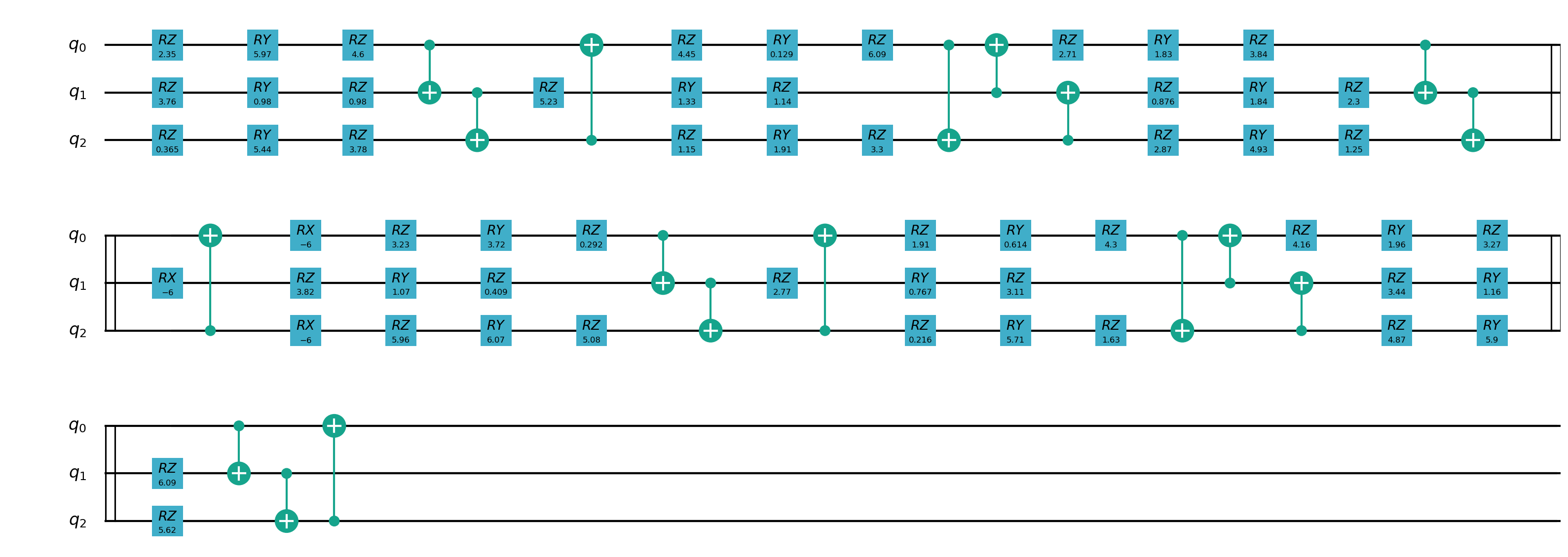
The network training results are:
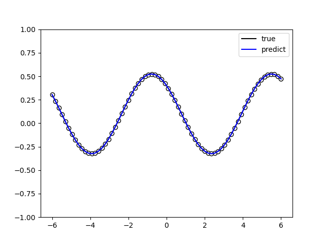
The network training loss is:
start training..............
epoch:0, #### loss:0.0037272341538482578
epoch:1, #### loss:5.271130586635309e-05
epoch:2, #### loss:4.714951917250687e-07
epoch:3, #### loss:1.0968826371082763e-08
epoch:4, #### loss:2.1258629738507562e-10
Expressive power of quantum circuits
In the paper Expressibility and entangling capability of parameterized quantum circuits for hybrid quantum-classical algorithms, The authors propose a method for expressiveness quantification based on the fidelity probability distribution between neural network output states. For any quantum neural network \(U(\vec{\theta})\) , sample the neural network parameters twice (set to \(\vec{\phi}\) and \(\vec{\psi }\) ), Then the fidelity between the output states of two quantum circuits \(F=|\langle0|U(\vec{\phi})^\dagger U(\vec{\psi})|0\rangle|^ 2\) obeys a probability distribution:
The literature points out that when the quantum neural network \(U\) can be uniformly distributed on all unitary matrices (at this time, it is called \(U\) obeys Haar distribution), the probability distribution of fidelity \(P_\text{Haar }(f)\) satisfies:
K-L divergence (also known as relative entropy) in statistical mathematics measures the difference between two probability distributions. The K-L divergence between two discrete probability distributions \(P,Q\) is defined as:
If the fidelity distribution of the quantum neural network output is recorded as \(P_\text{QNN}(f)\), then the expressive ability of the quantum neural network is defined as \(P_\text{QNN}(f) ` and :math:`P_\text{Haar}(f)\) K-L divergence between:
Therefore, when \(P_\text{QNN}(f)\) is closer to \(P_\text{Haar}(f)\), \(\text{Expr}\) will be smaller (more tends to 0), The expressive ability of the quantum neural network is also stronger; conversely, the larger the \(\text{Expr}\) is, the weaker the expressive ability of the quantum neural network is. We can directly compute single-bit quantum neural networks expressiveness according to this definition \(R_Y(\theta)\) , \(R_Y(\theta_1)R_Z(\theta_2)\) and \(R_Y(\theta_1)R_Z(\theta_2)R_Y(\theta_3)\):
The following uses VQNet to demonstrate the quantum circuit expression capabilities of HardwareEfficientAnsatz at different depths (1, 2, 3).
import numpy as np
import matplotlib.pyplot as plt
from matplotlib.ticker import FuncFormatter
from scipy import integrate
from scipy.linalg import sqrtm
from scipy.stats import entropy
import pyqpanda as pq
import numpy as np
from pyvqnet.qnn.ansatz import HardwareEfficientAnsatz
from pyvqnet.tensor import tensor
from pyvqnet.qnn.quantum_expressibility.quantum_express import fidelity_of_cir, fidelity_harr_sample
num_qubit = 1  # the number of qubit
num_sample = 2000  # the number of sample
outputs_y = list()  # save QNN outputs
# plot histgram
def plot_hist(data, num_bin, title_str):
    def to_percent(y, position):
        return str(np.around(y * 100, decimals=2)) + '%'
    plt.hist(data,
            weights=[1. / len(data)] * len(data),
            bins=np.linspace(0, 1, num=num_bin),
            facecolor="blue",
            edgecolor="black",
            alpha=0.7)
    plt.xlabel("Fidelity")
    plt.ylabel("frequency")
    plt.title(title_str)
    formatter = FuncFormatter(to_percent)
    plt.gca().yaxis.set_major_formatter(formatter)
    plt.show()
def cir(num_qubits, depth):
    machine = pq.CPUQVM()
    machine.init_qvm()
    qlist = machine.qAlloc_many(num_qubits)
    az = HardwareEfficientAnsatz(num_qubits, ["rx", "RY", "rz"],
                                qlist,
                                entangle_gate="cnot",
                                entangle_rules="linear",
                                depth=depth)
    w = tensor.QTensor(
        np.random.uniform(size=[az.get_para_num()], low=0, high=2 * np.pi))
    cir1 = az.create_ansatz(w)
    return cir1, machine, qlist
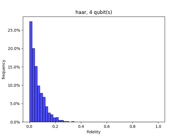
# Set circuit width and maximum depth
num_qubit = 4
max_depth = 3
# Calculate the fidelity distribution corresponding to Haar sampling

flist, p_haar, theory_haar = fidelity_harr_sample(num_qubit, num_sample)
title_str = "haar, %d qubit(s)" % num_qubit
plot_hist(flist, 50, title_str)
Expr_cel = list()
# Calculate the expressive power of neural networks with different depths
for DEPTH in range(1, max_depth + 1):
    print("Sampling circuit at depth %d..." % DEPTH)
    f_list, p_cel = fidelity_of_cir(HardwareEfficientAnsatz, num_qubit, DEPTH,
                                    num_sample)
    title_str = f"HardwareEfficientAnsatz, {num_qubit} qubit(s) {DEPTH} layer(s)"
    plot_hist(f_list, 50, title_str)
    expr = entropy(p_cel, theory_haar)
    Expr_cel.append(expr)
# Compare the expressive power of neural networks of different depths
print(
    f"The expressive power of neural networks with depths 1, 2, and 3 are { np.around(Expr_cel, decimals=4)}, the smaller the better.", )
plt.plot(range(1, max_depth + 1), Expr_cel, marker='>')
plt.xlabel("depth")
plt.yscale('log')
plt.ylabel("Expr.")
plt.xticks(range(1, max_depth + 1))
plt.title("Expressibility vs Circuit Depth")
plt.show()
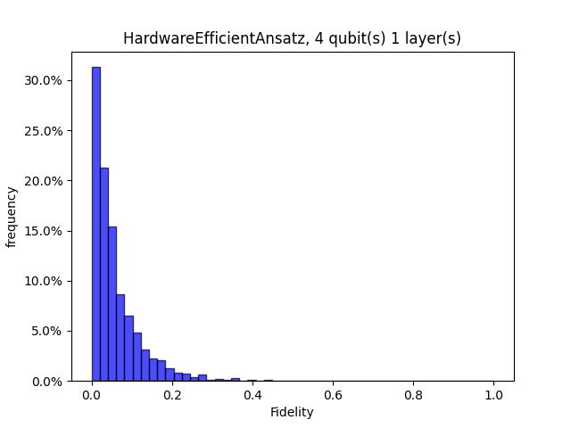
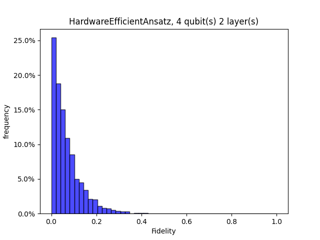
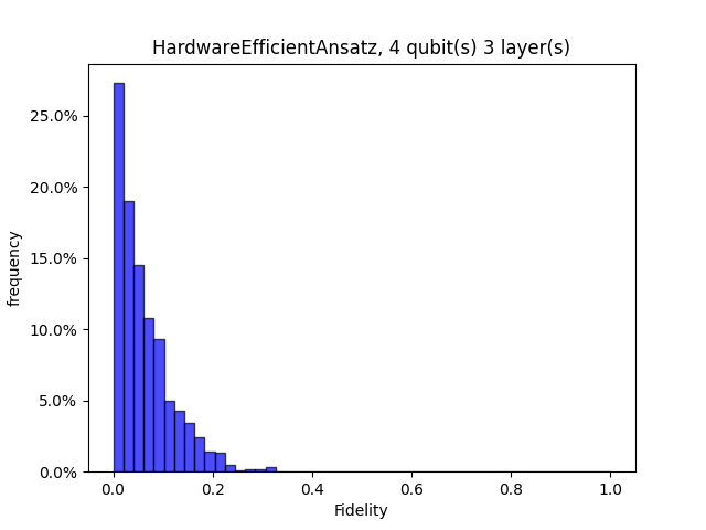
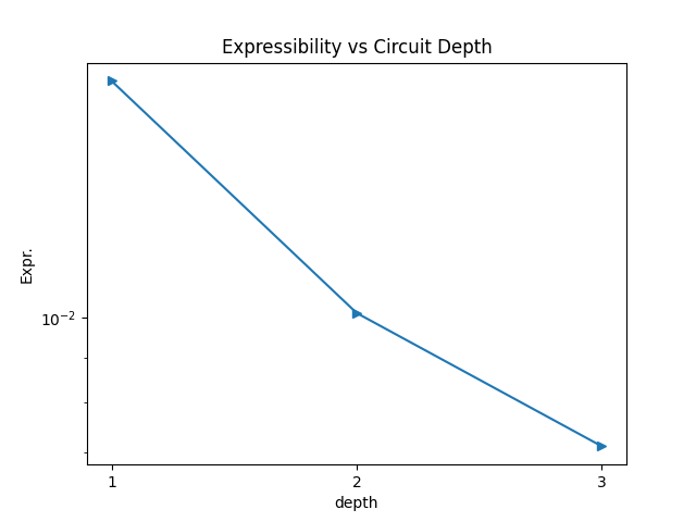
Quantum Perceptron
Artificial neural networks are the heart of machine learning algorithms and artificial intelligence protocols. Historically, the simplest implementation of an artificial neuron traces back to the classical Rosenblatt’s perceptron, but its long term practical applications may be hindered by the fast scaling up of computational complexity, especially relevant for the training of multilayered perceptron networks. Here we refer to the paper An Artificial Neuron Implemented on an Actual Quantum Processor introduce a quantum information-based algorithm implementing the quantum computer version of a perceptron, which shows exponential advantage in encoding resources over alternative realizations.
For this quantum perceptron, the data processed is a string of 0 1 binary bits. The goal is to identify patterns that are shaped like a w cross as shown in the figure below.

It is encoded using a binary bit string, where black is 0 and white is 1, so that w is encoded as (1, 1, 1, 1, 1, 1, 0, 1, 1, 0, 0, 0, 1, 1, 0, 1). A total of 16-bit strings can be encoded into the sign of the amplitude of the 4-bit quantum state. The sign is 0 for negative numbers, and 1 for positive numbers. Through the above encoding method, our algorithm input is converted into a 16-bit binary string. Such non-repetitive binary strings can respectively correspond to specific input \(U_i\) .
The circuit structure of the quantum perceptron proposed in this paper is as follows:
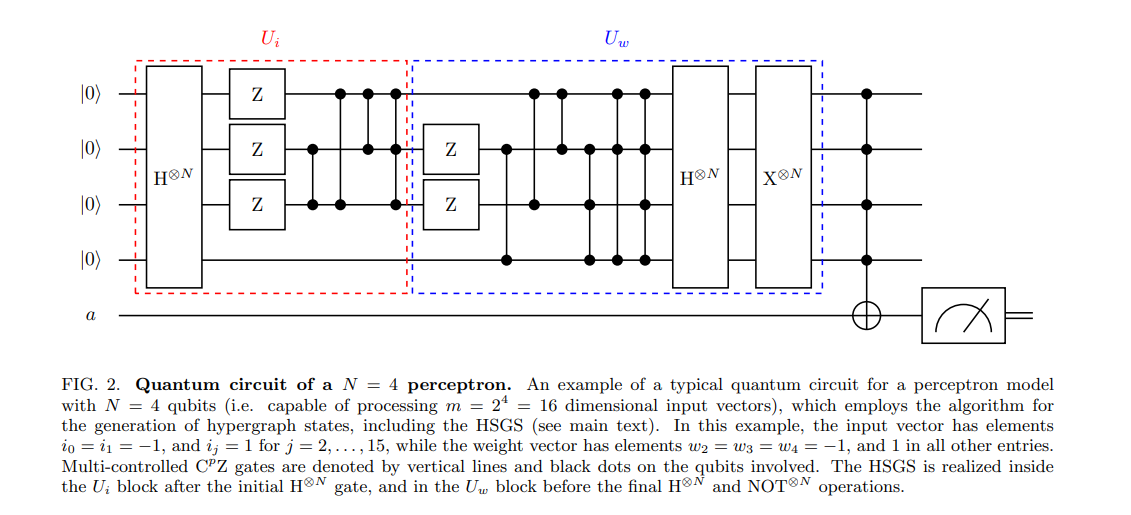
The coding circuit \(U_i\) is constructed on bits 0~3, including multiple controlled \(CZ\) , \(CNOT\) gates, and \(H\) gates; the weight conversion circuit \(U_w\) is constructed immediately after \(U_i\) , which is also composed of controlled gates and \(H\) gates. \(U_i\) can be used to perform unitary matrix transformations to encode data into quantum states:
Use the unitary matrix transformation \(U_w\) to compute the inner product between the input and the weights:
The normalized activation probability values for \(U_i\) and \(U_w\) can be obtained by using a multi-controlled NOT gate with target bits on auxiliary bits, and using some subsequent \(H\) gates, \(X\) gates, and \(CX\) gates as activation functions:
When the binary string of the input i is exactly the same as w, the normalized probability value should be the largest.
VQNet provides the QuantumNeuron module to implement this algorithm. First initialize a quantum perceptron QuantumNeuron.
perceptron = QuantumNeuron()
Use the gen_4bitstring_data interface to generate various data in the paper and its category labels.
training_label, test_label = perceptron.gen_4bitstring_data()
Using the train interface to traverse all the data, you can get the last trained quantum perceptron circuit \(U_w\).
trained_para = perceptron.train(training_label, test_label)
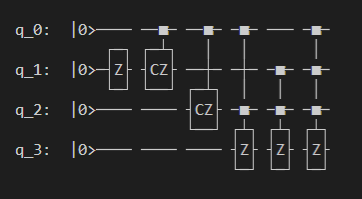
On the test data, the accuracy results on the test data can be obtained
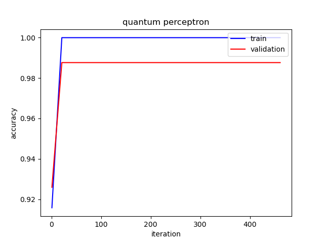
Stochastic parameter shift algorithm
In the quantum variational circuit, it is a common method to use the parameter shift method parameter-shift to calculate the gradient of the quantum parameter. The parameter shift method is not universally applicable to all quantum parametric logic gates. In cases where it does not hold (or is not known to hold), we either have to factorize the gates into compatible gates, or use an alternative estimator of the gradient, such as a finite difference approximation. However, both alternatives may have drawbacks due to increased circuit complexity or potential errors in gradient values. Banchi and Crooks 1 discovered a Stochastic Parameter-Shift Rule that can be applied to any unitary matrix quantum logic gate.
The following shows an example of applying VQNet to calculate the gradient using the random parameter offset method for a quantum variational circuit. An example line definition is as follows:
import pyqpanda as pq
import numpy as np
from pyvqnet.qnn.measure import expval
from scipy.linalg import expm
import matplotlib
try:
    matplotlib.use('TkAgg')
except:
    pass
import matplotlib.pyplot as plt
machine = pq.init_quantum_machine(pq.QMachineType.CPU)
q = machine.qAlloc_many(2)
c = machine.cAlloc_many(2)
# some basic Pauli matrices
I = np.eye(2)
X = np.array([[0, 1], [1, 0]])
Y = np.array([[0, -1j], [1j, 0]])
Z = np.array([[1, 0], [0, -1]])
def Generator(theta1, theta2, theta3):
    G = theta1.item() * np.kron(X, I) - \
        theta2 * np.kron(Z, X) + \
        theta3 * np.kron(I, X)
    return G
def pq_demo_circuit(gate_pars):
    G = Generator(*gate_pars)
    G = expm(-1j * G)
    x = G.flatten().tolist()
    cir = pq.matrix_decompose(q, x)
    m_prog = pq.QProg()
    m_prog.insert(cir)
    pauli_dict = {'Z0': 1}
    exp2 = expval(machine, m_prog, pauli_dict, q)
    return exp2
- The stochastic parameter shift method first randomly samples a variable
s from the uniform distribution of [0,1], and then performs the following unitary matrix transformation on the lines:
\(e^{i(1-s)(\hat{H} + \theta\hat{V})}\)
\(e^{+i\tfrac{\pi}{4}\hat{V}}\)
\(e^{is(\hat{H} + \theta\hat{V})}\)
where \(\hat{V}\) is a tensor product of Pauli operators, and \(\hat{H}\) is a linear combination of any Pauli operator tensor product. We define the expected value of the observabley obtained at this time as \(\langle r_+ \rangle\).
def pq_SPSRgates(gate_pars, s, sign):
    G = Generator(*gate_pars)
    # step a)
    G1 = expm(1j * (1 - s) * G)
    x = G1.flatten().tolist()
    cir = pq.matrix_decompose(q, x)
    m_prog = pq.QProg()
    m_prog.insert(cir)
    # step b)
    G2 = expm(1j * sign * np.pi / 4 * X)
    x = G2.flatten().tolist()
    cir = pq.matrix_decompose(q[0], x)
    m_prog.insert(cir)
    # step c)
    G3 = expm(1j * s * G)
    x = G3.flatten().tolist()
    cir = pq.matrix_decompose(q, x)
    m_prog.insert(cir)
    pauli_dict = {'Z0': 1}
    exp2 = expval(machine, m_prog, pauli_dict, q)
    return exp2
Change \(\tfrac{\pi}{4}\) in the previous step to \(-\tfrac{\pi}{4}\), Repeat operations a, b, c to obtain observable
The gradient formula calculated by the stochastic parameter shift algorithm is as follows:
\[\mathbb{E}_{s\in\mathcal{U}[0,1]}[\langle r_+ \rangle - \langle r_-\rangle]\]
In the following figure, the gradient of the parameter \(\theta_1\) is showed, using the stochastic parameter shift method. It can be seen that the observable is expected to conform to the functional form of \(\cos(2\theta_1)\); and the gradient is calculated using the random parameter shift method,
Meets \(-2\sin(2\theta_1)\) , which is exactly the differential of \(\cos(2\theta_1)\).
theta2, theta3 = -0.15, 1.6
angles = np.linspace(0, 2 * np.pi, 50)
pos_vals = np.array([[
    pq_SPSRgates([theta1, theta2, theta3], s=s, sign=+1)
    for s in np.random.uniform(size=10)
] for theta1 in angles])
neg_vals = np.array([[
    pq_SPSRgates([theta1, theta2, theta3], s=s, sign=-1)
    for s in np.random.uniform(size=10)
] for theta1 in angles])
# Plot the results
evals = [pq_demo_circuit([theta1, theta2, theta3]) for theta1 in angles]
spsr_vals = (pos_vals - neg_vals).mean(axis=1)
plt.plot(angles, evals, 'b', label="Expectation Value")
plt.plot(angles, spsr_vals, 'r', label="Stochastic parameter-shift rule")
plt.xlabel("theta1")
plt.legend()
plt.title("VQNet")
plt.show()
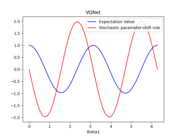
Doubly Stochastic Gradient Descent
In variational quantum algorithms, parameterized quantum circuits are optimized by classical gradient descent to minimize the expected function value. Although the expected value can be calculated analytically in classical simulator, on quantum hardware the program is limited to sampling from the expected value; as the number of samples and the number of shots increase, the expected value obtained in this way will converge to the theoretical expected value, but may always be accurate value. Sweke et al. found a double stochastic gradient descent method in the paper. In this paper, they show that quantum gradient descent, which uses a finite number of measurement samples (or shots) to estimate gradients, is a form of stochastic gradient descent. Furthermore, if the optimization involves a linear combination of expected values (such as VQE), sampling from the terms in that linear combination can further reduce the required time complexity.
VQNet implements an example of this algorithm: solving the ground state energy of the target Hamiltonian using VQE. Note that here we set the number of shots for quantum circuit observations to only 1.
import numpy as np
import pyqpanda as pq
from pyvqnet.qnn.template import StronglyEntanglingTemplate
from pyvqnet.qnn.measure import Hermitian_expval
from pyvqnet.qnn import QuantumLayerV2
from pyvqnet.optim import SGD
import pyvqnet._core as _core
from pyvqnet.tensor import QTensor
from matplotlib import pyplot as plt
num_layers = 2
num_wires = 2
eta = 0.01
steps = 200
n = 1
param_shape = [2, 2, 3]
shots = 1
H = np.array([[8, 4, 0, -6], [4, 0, 4, 0], [0, 4, 8, 0], [-6, 0, 0, 0]])
init_params = np.random.uniform(low=0,
                                high=2 * np.pi,
                                size=param_shape).astype(np.float32)
# some basic Pauli matrices
I = np.eye(2)
X = np.array([[0, 1], [1, 0]])
Y = np.array([[0, -1j], [1j, 0]])
Z = np.array([[1, 0], [0, -1]])

def pq_circuit(params):
    params = params.reshape(param_shape)
    num_qubits = 2
    machine = pq.CPUQVM()
    machine.init_qvm()
    qubits = machine.qAlloc_many(num_qubits)
    circuit = StronglyEntanglingTemplate(params, num_qubits=num_qubits)
    qcir = circuit.create_circuit(qubits)
    prog = pq.QProg()
    prog.insert(qcir)
    machine.directly_run(prog)
    result = machine.get_qstate()
    return result
- The Hamiltonian in this example is a Hermitian matrix,
which we can always represent as a sum of Pauli matrices.
and
Substituting into the above formula, we can see that
To perform “doubly stochastic” gradient descent, we simply apply the stochastic gradient descent method, but additionally uniformly sample a subset of the Hamiltonian expectation at each optimization step. The vqe_func_analytic() function uses parameter shift to calculate theoretical gradients, and vqe_func_shots() uses random sampled values and randomly sampled Hamiltonian expectation subsets for “doubly stochastic” gradient calculations.
terms = np.array([
    2 * np.kron(I, X),
    4 * np.kron(I, Z),
    -np.kron(X, X),
    5 * np.kron(Y, Y),
    2 * np.kron(Z, X),
])
def vqe_func_analytic(input, init_params):
    qstate = pq_circuit(init_params)
    expval = Hermitian_expval(H, qstate, [0, 1], 2)
    return  expval
def vqe_func_shots(input, init_params):
    qstate = pq_circuit(init_params)
    idx = np.random.choice(np.arange(5), size=n, replace=False)
    A = np.sum(terms[idx], axis=0)
    expval = Hermitian_expval(A, qstate, [0, 1], 2, shots)
    return 4 + (5 / 1) * expval
Use VQNet for parameter optimization, and compare the curve of the loss function. Since the double stochastic gradient descent method only calculates the partial Pauli operator sum of H each time, Therefore, the average value can be used to represent the expected result of the final observation. Here, the moving average moving_average() is used for calculation.
##############################################################################
# Optimizing the circuit using gradient descent via the parameter-shift rule:
qlayer_ana = QuantumLayerV2(vqe_func_analytic, 2*2*3 )
qlayer_shots = QuantumLayerV2(vqe_func_shots, 2*2*3 )
cost_sgd = []
cost_dsgd = []
temp = _core.Tensor(init_params)
_core.vqnet.copyTensor(temp, qlayer_ana.m_para.data)
opti_ana = SGD(qlayer_ana.parameters())

_core.vqnet.copyTensor(temp, qlayer_shots.m_para.data)
opti_shots = SGD(qlayer_shots.parameters())

for i in range(steps):
    opti_ana.zero_grad()
    loss = qlayer_ana(QTensor([[1.0]]))
    loss.backward()
    cost_sgd.append(loss.item())
    opti_ana._step()
for i in range(steps+50):
    opti_shots.zero_grad()
    loss = qlayer_shots(QTensor([[1.0]]))
    loss.backward()
    cost_dsgd.append(loss.item())
    opti_shots._step()
def moving_average(data, n=3):
    ret = np.cumsum(data, dtype=np.float64)
    ret[n:] = ret[n:] - ret[:-n]
    return ret[n - 1:] / n
ta = moving_average(np.array(cost_dsgd), n=50)
ta = ta[:-26]
average = np.vstack([np.arange(25, 200),ta ])
final_param = qlayer_shots.parameters()[0].to_numpy()
print("Doubly stochastic gradient descent min energy = ", vqe_func_analytic(QTensor([1]),final_param))
final_param  = qlayer_ana.parameters()[0].to_numpy()
print("stochastic gradient descent min energy = ", vqe_func_analytic(QTensor([1]),final_param))
plt.plot(cost_sgd, label="Vanilla gradient descent")
plt.plot(cost_dsgd, ".", label="Doubly QSGD")
plt.plot(average[0], average[1], "--", label="Doubly QSGD (moving average)")
plt.ylabel("Cost function value")
plt.xlabel("Optimization steps")
plt.xlim(-2, 200)
plt.legend()
plt.show()
#Doubly stochastic gradient descent min energy =  -4.337801834749975
#stochastic gradient descent min energy =  -4.531484333030544
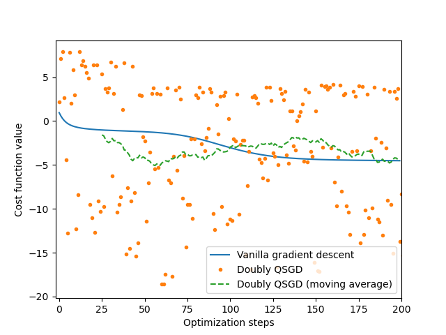
Barren plateaus
In the training of classical neural networks, gradient-based optimization methods not only encounter the problem of local minima, It also encounters geometric structures such as saddle points where the gradient is close to zero. Correspondingly, the barren plateau effect (plataus) also exists in the quantum neural network. This peculiar phenomenon was first discovered by McClean et al. in 2018 Barren plateaus in quantum neural network training landscapes. Simply put, the optimization landscape becomes very flat when you choose a random circuit structure that satisfies a certain level of complexity, This makes it difficult for gradient descent based optimization methods to find the global minimum . For most variational quantum algorithms (VQE, etc.), this phenomenon means that when the number of qubits increases, Circuits with random structures may not work well. This will turn the optimization surface corresponding to the well-designed loss function into a huge platform, Make the training of quantum neural networks more difficult. The initial value randomly found by the model is difficult to escape from this platform, and the convergence speed of gradient descent will be very slow.
This case mainly uses VQNet to display the barren plateau phenomenon, and uses the gradient analysis function to analyze the parameter gradient in the user-defined quantum neural network.
The following code builds the following random circuit according to the similar method mentioned in the original paper:
First act on all qubits with a rotation about the Y-axis of the Bloch sphere \(\pi/4\).
The rest of the structures add up to form a module (Block), each module is divided into two layers:
The first layer builds a random revolving door, where \(R \in \{R_x, R_y, R_z\}\).
The second layer consists of CZ gates acting on every two adjacent qubits.
The circuit code is shown in the rand_circuit_pq function.
After we have determined the structure of the circuit, we also need to define a loss function (loss function) to determine the optimization surface. As mentioned in the original paper, we use the loss function commonly used in the VQE algorithm:
The unitary matrix \(U(\boldsymbol{\theta})\) is the quantum neural network with random structure we built in the previous part. Hamiltonian \(H = |00\cdots 0\rangle\langle00\cdots 0|\). In this case, the above VQE algorithm is constructed on different qubit numbers, and 200 sets of random network structures and different random initial parameters are generated. The gradient of the parameters in the line with parameters is calculated according to the paramter-shift algorithm. Then count the average and variance of the 200 gradients of the variational parameters obtained.
The following example analyzes the last of the variable quantum parameters, and readers can also modify it to other reasonable values. Through the operation, it is not difficult for readers to find that as the number of qubits increases, the variance of the gradient of the quantum parameters becomes smaller and smaller, and the mean value is closer to 0.
"""
barren plateau
"""
import pyqpanda as pq
import numpy as np
import matplotlib.pyplot as plt

from pyvqnet.qnn import Hermitian_expval, grad

param_idx = -1
gate_set = [pq.RX, pq.RY, pq.RZ]


def rand_circuit_pq(params, num_qubits):
    cir = pq.QCircuit()
    machine = pq.CPUQVM()
    machine.init_qvm()
    qlist = machine.qAlloc_many(num_qubits)

    for i in range(num_qubits):
        cir << pq.RY(
            qlist[i],
            np.pi / 4,
        )

    random_gate_sequence = {
        i: np.random.choice(gate_set)
        for i in range(num_qubits)
    }
    for i in range(num_qubits):
        cir << random_gate_sequence[i](qlist[i], params[i])

    for i in range(num_qubits - 1):
        cir << pq.CZ(qlist[i], qlist[i + 1])

    prog = pq.QProg()
    prog.insert(cir)
    machine.directly_run(prog)
    result = machine.get_qstate()

    H = np.zeros((2**num_qubits, 2**num_qubits))
    H[0, 0] = 1
    expval = Hermitian_expval(H, result, [i for i in range(num_qubits)],
                            num_qubits)

    return expval


qubits = [2, 3, 4, 5, 6]
variances = []
num_samples = 200
means = []
for num_qubits in qubits:
    grad_vals = []
    for i in range(num_samples):
        params = np.random.uniform(0, np.pi, size=num_qubits)
        g = grad(rand_circuit_pq, params, num_qubits)

        grad_vals.append(g[-1])
    variances.append(np.var(grad_vals))
    means.append(np.mean(grad_vals))
variances = np.array(variances)
means = np.array(means)
qubits = np.array(qubits)


plt.figure()

plt.plot(qubits, variances, "v-")

plt.xlabel(r"N Qubits")
plt.ylabel(r"variance")
plt.show()


plt.figure()
# Plot the straight line fit to the semilog
plt.plot(qubits, means, "v-")

plt.xlabel(r"N Qubits")
plt.ylabel(r"means")

plt.show()
The figure below shows how the mean value of the parameter gradient varies with the number of qubits. As the number of qubits increases, the parameter gradient approaches 0.
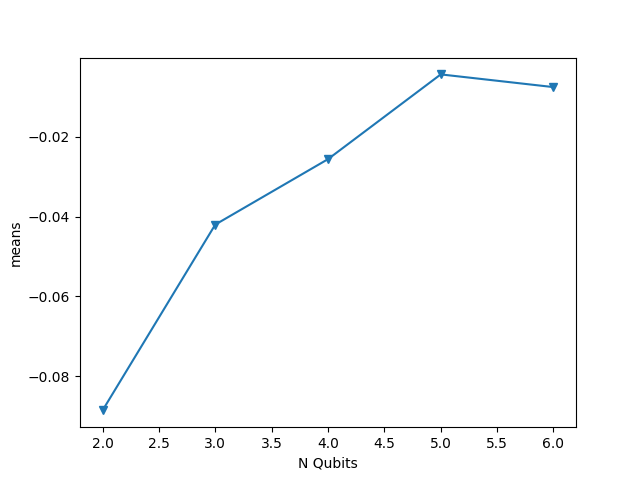
The figure below shows how the variance of the parameter gradient varies with the number of qubits, and the parameter gradient hardly changes as the number of qubits increases. It can be foreseen that the quantum circuit built by any parametric logic gate will be difficult to update in the case of arbitrary parameter initialization when the qubits are improved.
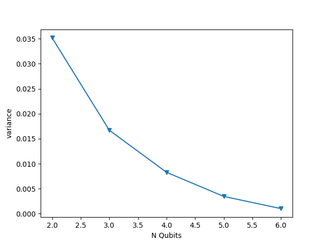
Gradient based pruning
The following example implements the algorithm in the paper Towards Efficient On-Chip Training of Quantum Neural Networks. By carefully studying the process of parameters in the quantum variational circuit, the researchers observed that small gradients often have large relative changes or even wrong directions under quantum noise. Also, not all gradient computations are necessary for the training process, especially for small magnitude gradients. Inspired by this, the researchers propose a probabilistic gradient pruning method to predict and only compute gradients with high reliability. The approach reduces noise effects and also saves the number of circuits needed to run on a real quantum machine.
In the gradient based pruning algorithm, for the optimization process of parameters, two stages of accumulation window and pruning window are divided, and all training periods are divided into a repeated accumulation window and then a pruning window. There are three important hyperparameters in the probabilistic gradient pruning method:
Cumulative window width \(\omega_a\) ,
trim ratio \(r\) ,
Trim window width \(\omega_p\) .
In the accumulation window, THe researchers collect the gradient information in each training step. At each step of pruning the window, based on the information gathered from the accumulation window and the pruning ratio, the algorithm Probabilistically skips some gradient computations.
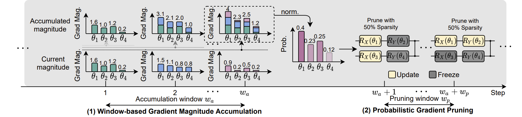
The pruning ratio \(r\) , the cumulative window width \(\omega_a\) and the pruning window width \(\omega_p\) respectively determine the reliability of the gradient trend evaluation. Thus, the percentage time saved by our probabilistic gradient pruning method is \(r\tfrac{\omega_p}{\omega_a +\omega_p}\times 100\%\). The following is the application of the QVC classification example using the gradient pruning algorithm.
import random
import numpy as np
import pyqpanda as pq

from pyvqnet.data import data_generator as dataloader
from pyvqnet.nn.module import Module
from pyvqnet.optim import sgd
from pyvqnet.qnn.quantumlayer import QuantumLayer
from pyvqnet.nn.loss import CategoricalCrossEntropy
from pyvqnet.tensor.tensor import QTensor
from pyvqnet.qnn import Gradient_Prune_Instance
random.seed(1234)

qvc_train_data = [
    0, 1, 0, 0, 1, 0, 1, 0, 1, 0, 0, 1, 1, 0, 0, 0, 1, 1, 1, 1, 1, 0, 0, 0, 1,
    1, 0, 0, 1, 0, 1, 0, 1, 0, 0, 1, 0, 1, 1, 1, 1, 1, 0, 0, 0, 1, 1, 0, 1, 1,
    1, 1, 1, 0, 1, 1, 1, 1, 1, 0
]
qvc_test_data = [0, 0, 0, 0, 0, 0, 0, 0, 1, 1, 0, 0, 1, 0, 1, 0, 0, 1, 1, 0]


def qvc_circuits(x, weights, qlist, clist, machine):
    """
    Quantum circuits run function
    """
    def get_cnot(nqubits):
        cir = pq.QCircuit()
        for i in range(len(nqubits) - 1):
            cir.insert(pq.CNOT(nqubits[i], nqubits[i + 1]))
        cir.insert(pq.CNOT(nqubits[len(nqubits) - 1], nqubits[0]))
        return cir

    def build_circult(weights, xx, nqubits):
        def Rot(weights_j, qubits):
            circult = pq.QCircuit()
            circult.insert(pq.RZ(qubits, weights_j[0]))
            circult.insert(pq.RY(qubits, weights_j[1]))
            circult.insert(pq.RZ(qubits, weights_j[2]))
            return circult

        def basisstate():
            circult = pq.QCircuit()
            for i in range(len(nqubits)):
                if xx[i] == 1:
                    circult.insert(pq.X(nqubits[i]))
            return circult

        circult = pq.QCircuit()
        circult.insert(basisstate())

        for i in range(weights.shape[0]):

            weights_i = weights[i, :, :]
            for j in range(len(nqubits)):
                weights_j = weights_i[j]
                circult.insert(Rot(weights_j, nqubits[j]))
            cnots = get_cnot(nqubits)
            circult.insert(cnots)

        circult.insert(pq.Z(nqubits[0]))

        prog = pq.QProg()

        prog.insert(circult)
        return prog

    weights = weights.reshape([2, 4, 3])
    prog = build_circult(weights, x, qlist)
    prob = machine.prob_run_dict(prog, qlist[0], -1)
    prob = list(prob.values())

    return prob


def qvc_circuits2(x, weights, qlist, clist, machine):
    """
    Quantum circuits run function
    """
    prog = pq.QProg()
    circult = pq.QCircuit()
    circult.insert(pq.RZ(qlist[0], x[0]))
    circult.insert(pq.RZ(qlist[1], x[1]))
    circult.insert(pq.CNOT(qlist[0], qlist[1]))
    circult.insert(pq.CNOT(qlist[1], qlist[2]))
    circult.insert(pq.CNOT(qlist[2], qlist[3]))
    circult.insert(pq.RY(qlist[0], weights[0]))
    circult.insert(pq.RY(qlist[1], weights[1]))
    circult.insert(pq.RY(qlist[2], weights[2]))

    circult.insert(pq.CNOT(qlist[0], qlist[1]))
    circult.insert(pq.CNOT(qlist[1], qlist[2]))
    circult.insert(pq.CNOT(qlist[2], qlist[3]))
    prog.insert(circult)
    prob = machine.prob_run_dict(prog, qlist[0], -1)
    prob = list(prob.values())

    return prob

class Model(Module):
    def __init__(self):
        super(Model, self).__init__()
        self.qvc = QuantumLayer(qvc_circuits, 24, "cpu", 4)

    def forward(self, x):
        y = self.qvc(x)
        #y = self.qvc2(y)
        return y


def get_data(dataset_str):
    """
    Tranform data to valid form
    """
    if dataset_str == "train":
        datasets = np.array(qvc_train_data)

    else:
        datasets = np.array(qvc_test_data)

    datasets = datasets.reshape([-1, 5])
    data = datasets[:, :-1]
    label = datasets[:, -1].astype(int)
    label = np.eye(2)[label].reshape(-1, 2)
    return data, label


def get_accuary(result, label):
    result, label = np.array(result.data), np.array(label.data)
    score = np.sum(np.argmax(result, axis=1) == np.argmax(label, 1))
    return score
We use the Gradient_Prune_Instance class, and enter 24 as the number of parameters param_num.
The cropping ratio prune_ratio is 0.5,
the cumulative window size accumulation_window_size is 4,
and the pruning window pruning_window_size is 2.
When backpropagating part of the code each run, before the optimizer step,
Run the step function of Gradient_Prune_Instance.
def run():
    """
    Main run function
    """
    model = Model()

    optimizer = sgd.SGD(model.parameters(), lr=0.5)
    batch_size = 3
    epoch = 10
    loss = CategoricalCrossEntropy()
    print("start training..............")
    model.train()

    datas, labels = get_data("train")
    print(datas)
    print(labels)
    print(datas.shape)


    GBP_HELPER = Gradient_Prune_Instance(param_num = 24,prune_ratio=0.5,accumulation_window_size=4,pruning_window_size=2)
    for i in range(epoch):
        count = 0
        sum_loss = 0
        accuary = 0
        t = 0
        for data, label in dataloader(datas, labels, batch_size, False):
            optimizer.zero_grad()
            data, label = QTensor(data), QTensor(label)

            result = model(data)

            loss_b = loss(label, result)

            loss_b.backward()

            GBP_HELPER.step(model.parameters())
            optimizer._step()
            sum_loss += loss_b.item()
            count += batch_size
            accuary += get_accuary(result, label)
            t = t + 1

        print(
            f"epoch:{i}, #### loss:{sum_loss/count} #####accuray:{accuary/count}"
        )
    print("start testing..............")
    model.eval()
    count = 0

    test_data, test_label = get_data("test")
    test_batch_size = 1
    accuary = 0
    sum_loss = 0
    for testd, testl in dataloader(test_data, test_label, test_batch_size):
        testd = QTensor(testd)
        test_result = model(testd)
        test_loss = loss(testl, test_result)
        sum_loss += test_loss
        count += test_batch_size
        accuary += get_accuary(test_result, testl)
    print(
        f"test:--------------->loss:{sum_loss/count} #####accuray:{accuary/count}"
    )


if __name__ == "__main__":

    run()

# epoch:0, #### loss:0.2255942871173223 #####accuray:0.5833333333333334
# epoch:1, #### loss:0.1989427705605825 #####accuray:1.0
# epoch:2, #### loss:0.16489211718241373 #####accuray:1.0
# epoch:3, #### loss:0.13245886812607446 #####accuray:1.0
# epoch:4, #### loss:0.11463981121778488 #####accuray:1.0
# epoch:5, #### loss:0.1078591321905454 #####accuray:1.0
# epoch:6, #### loss:0.10561319688955943 #####accuray:1.0
# epoch:7, #### loss:0.10483601937691371 #####accuray:1.0
# epoch:8, #### loss:0.10457512239615123 #####accuray:1.0
# epoch:9, #### loss:0.10448987782001495 #####accuray:1.0
# start testing..............
# test:--------------->loss:[0.3134713] #####accuray:1.0
Model training using quantum computing layer in VQNet
The following are some examples of using VQNet inrerface for quantum machine learning QuantumLayer , NoiseQuantumLayer .
Model training using quantumlayer in VQNet
import sys,os
from pyvqnet.nn.module import Module
from pyvqnet.optim import sgd
import numpy as np

from pyvqnet.data import data_generator as dataloader
from pyvqnet.nn.linear import Linear
from pyvqnet.nn.loss import CategoricalCrossEntropy

from pyvqnet.tensor.tensor import QTensor
import random
import pyqpanda as pq
from pyvqnet.qnn.quantumlayer import QuantumLayer
from pyqpanda import *
random.seed(1234)

qvc_train_data = [0,1,0,0,1,
0, 1, 0, 1, 0,
0, 1, 1, 0, 0,
0, 1, 1, 1, 1,
1, 0, 0, 0, 1,
1, 0, 0, 1, 0,
1, 0, 1, 0, 0,
1, 0, 1, 1, 1,
1, 1, 0, 0, 0,
1, 1, 0, 1, 1,
1, 1, 1, 0, 1,
1, 1, 1, 1, 0]
qvc_test_data= [0, 0, 0, 0, 0,
0, 0, 0, 1, 1,
0, 0, 1, 0, 1,
0, 0, 1, 1, 0]

def qvc_circuits(input,weights,qlist,clist,machine):

    def get_cnot(nqubits):
        cir = pq.QCircuit()
        for i in range(len(nqubits)-1):
            cir.insert(pq.CNOT(nqubits[i],nqubits[i+1]))
        cir.insert(pq.CNOT(nqubits[len(nqubits)-1],nqubits[0]))
        return cir

    def build_circult(weights, xx, nqubits):

        def Rot(weights_j, qubits):
            circult = pq.QCircuit()
            circult.insert(pq.RZ(qubits, weights_j[0]))
            circult.insert(pq.RY(qubits, weights_j[1]))
            circult.insert(pq.RZ(qubits, weights_j[2]))
            return circult
        def basisstate():
            circult = pq.QCircuit()
            for i in range(len(nqubits)):
                if xx[i]==1:
                    circult.insert(pq.X(nqubits[i]))
            return circult

        circult = pq.QCircuit()
        circult.insert(basisstate())

        for i in range(weights.shape[0]):

            weights_i = weights[i,:,:]
            for j in range(len(nqubits)):
                weights_j = weights_i[j]
                circult.insert(Rot(weights_j,nqubits[j]))
            cnots = get_cnot(nqubits)
            circult.insert(cnots)

        circult.insert(pq.Z(nqubits[0]))

        prog = pq.QProg()

        prog.insert(circult)
        return prog

    weights = weights.reshape([2,4,3])
    prog = build_circult(weights,input,qlist)
    prob = machine.prob_run_dict(prog, qlist[0], -1)
    prob = list(prob.values())

    return prob

class Model(Module):
    def __init__(self):
        super(Model, self).__init__()
        self.qvc = QuantumLayer(qvc_circuits,24,"cpu",4)

    def forward(self, x):
        return self.qvc(x)

def get_data(dataset_str):
    if dataset_str == "train":
        datasets = np.array(qvc_train_data)

    else:
        datasets = np.array(qvc_test_data)

    datasets = datasets.reshape([-1,5])
    data = datasets[:,:-1]
    label = datasets[:,-1].astype(int)
    label = np.eye(2)[label].reshape(-1,2)
    return data, label

def get_accuary(result,label):
    result,label = np.array(result.data), np.array(label.data)
    score = np.sum(np.argmax(result,axis=1)==np.argmax(label,1))
    return score

def Run():

    model = Model()

    optimizer = sgd.SGD(model.parameters(),lr =0.5)
    batch_size = 3
    epoch = 10
    loss = CategoricalCrossEntropy()
    print("start training..............")
    model.train()

    datas,labels = get_data("train")
    print(datas)
    print(labels)
    print(datas.shape)
    for i in range(epoch):
        count=0
        sum_loss = 0
        accuary = 0
        t = 0
        for data,label in dataloader(datas,labels,batch_size,False):
            optimizer.zero_grad()
            data,label = QTensor(data), QTensor(label)

            result = model(data)

            loss_b = loss(label,result)
            loss_b.backward()
            optimizer._step()
            sum_loss += loss_b.item()
            count+=batch_size
            accuary += get_accuary(result,label)
            t = t + 1

        print(f"epoch:{i}, #### loss:{sum_loss/count} #####accuray:{accuary/count}")
    print("start testing..............")
    model.eval()
    count = 0
    test_data, test_label = get_data("test")
    test_batch_size = 1
    accuary = 0
    sum_loss = 0
    for testd,testl in dataloader(test_data,test_label,test_batch_size):
        testd = QTensor(testd)
        test_result = model(testd)
        test_loss = loss(testl,test_result)
        sum_loss += test_loss
        count+=test_batch_size
        accuary += get_accuary(test_result,testl)
    print(f"test:--------------->loss:{sum_loss/count} #####accuray:{accuary/count}")

if __name__=="__main__":

    Run()
Loss and accuracy results of the run:
start training..............
epoch:0, #### loss:[0.20585182] #####accuray:0.6
epoch:1, #### loss:[0.17479989] #####accuray:1.0
epoch:2, #### loss:[0.12679021] #####accuray:1.0
epoch:3, #### loss:[0.11088503] #####accuray:1.0
epoch:4, #### loss:[0.10598478] #####accuray:1.0
epoch:5, #### loss:[0.10482856] #####accuray:1.0
epoch:6, #### loss:[0.10453037] #####accuray:1.0
epoch:7, #### loss:[0.10445572] #####accuray:1.0
epoch:8, #### loss:[0.10442699] #####accuray:1.0
epoch:9, #### loss:[0.10442187] #####accuray:1.0
epoch:10, #### loss:[0.10442089] #####accuray:1.0
epoch:11, #### loss:[0.10442062] #####accuray:1.0
epoch:12, #### loss:[0.10442055] #####accuray:1.0
epoch:13, #### loss:[0.10442055] #####accuray:1.0
epoch:14, #### loss:[0.10442055] #####accuray:1.0
epoch:15, #### loss:[0.10442055] #####accuray:1.0
epoch:16, #### loss:[0.10442055] #####accuray:1.0

start testing..............
[0.3132616580]
test:--------------->loss:QTensor(0.3132616580, requires_grad=True) #####accuray:1.0
Model training using NoiseQuantumLayer in VQNet
Using NoiseQuantumLayer to build and train noisy quantum circuits using pyQPanda2’s noise virtual machine.
An example of a complete noisy quantum machine learning model is as follows:
import os
import numpy as np

from pyvqnet.nn.module import Module
from pyvqnet.nn.linear import Linear
from pyvqnet.nn.conv import Conv2D

from pyvqnet.nn import activation as F
from pyvqnet.nn.pooling import MaxPool2D
from pyvqnet.nn.loss import CategoricalCrossEntropy
from pyvqnet.optim.adam import Adam
from pyvqnet.data.data import data_generator
from pyvqnet.tensor import tensor

import pyqpanda as pq
from pyqpanda import *
from pyvqnet.qnn.quantumlayer import NoiseQuantumLayer
import matplotlib
try:
    matplotlib.use('TkAgg')
except:
    pass
import time
try:
    matplotlib.use('TkAgg')
except:
    pass

try:
    import urllib.request
except ImportError:
    raise ImportError('You should use Python 3.x')
import os.path
import gzip

url_base = 'https://ossci-datasets.s3.amazonaws.com/mnist/'
key_file = {
    'train_img':'train-images-idx3-ubyte.gz',
    'train_label':'train-labels-idx1-ubyte.gz',
    'test_img':'t10k-images-idx3-ubyte.gz',
    'test_label':'t10k-labels-idx1-ubyte.gz'
}


def _download(dataset_dir,file_name):
    file_path = dataset_dir + "/" + file_name

    if os.path.exists(file_path):
        with gzip.GzipFile(file_path) as f:
            file_path_ungz = file_path[:-3].replace('\\', '/')
            if not os.path.exists(file_path_ungz):
                open(file_path_ungz,"wb").write(f.read())
        return

    print("Downloading " + file_name + " ... ")
    urllib.request.urlretrieve(url_base + file_name, file_path)
    if os.path.exists(file_path):
            with gzip.GzipFile(file_path) as f:
                file_path_ungz = file_path[:-3].replace('\\', '/')
                file_path_ungz = file_path_ungz.replace('-idx', '.idx')
                if not os.path.exists(file_path_ungz):
                    open(file_path_ungz,"wb").write(f.read())
    print("Done")

def download_mnist(dataset_dir):
    for v in key_file.values():
        _download(dataset_dir,v)

#use qpanda to create quantum circuits
def circuit(weights,param,qubits,cbits,machine):

    circuit = pq.QCircuit()
    circuit.insert(pq.H(qubits[0]))
    circuit.insert(pq.RY(qubits[0], weights[0]))
    prog = pq.QProg()
    prog.insert(circuit)
    prog << measure_all(qubits, cbits)
    result = machine.run_with_configuration(prog, cbits, 100)
    counts = np.array(list(result.values()))
    states = np.array(list(result.keys())).astype(float)
    # Compute probabilities for each state
    probabilities = counts / 100
    # Get state expectation
    expectation = np.sum(states * probabilities)
    return expectation


class Net(Module):
    def __init__(self):
        super(Net, self).__init__()
        self.conv1 = Conv2D(input_channels=1, output_channels=6, kernel_size=(5, 5), stride=(1, 1), padding="valid")
        self.maxpool1 = MaxPool2D([2, 2], [2, 2], padding="valid")
        self.conv2 = Conv2D(input_channels=6, output_channels=16, kernel_size=(5, 5), stride=(1, 1), padding="valid")
        self.maxpool2 = MaxPool2D([2, 2], [2, 2], padding="valid")
        self.fc1 = Linear(input_channels=256, output_channels=64)
        self.fc2 = Linear(input_channels=64, output_channels=1)

        self.hybrid = NoiseQuantumLayer(circuit,1,"noise",1)
        self.fc3 = Linear(input_channels=1, output_channels=2)


    def forward(self, x):
        x = F.ReLu()(self.conv1(x))
        x = self.maxpool1(x)
        x = F.ReLu()(self.conv2(x))
        x = self.maxpool2(x)
        x = tensor.flatten(x, 1)
        x = F.ReLu()(self.fc1(x))
        x = self.fc2(x)
        x = self.hybrid(x)
        x = self.fc3(x)

        return x
The model is a hybrid quantum circuit and classical network model, in which the quantum circuit
part uses NoiseQuantumLayer to simulate the quantum circuit plus noise model. This model
is used to classify 0 and 1 handwritten digits in MNIST database.
def load_mnist(dataset="training_data", digits=np.arange(2), path="./"):
    import os, struct
    from array import array as pyarray
    download_mnist(path)
    if dataset == "training_data":
        fname_image = os.path.join(path, 'train-images.idx3-ubyte').replace('\\', '/')
        fname_label = os.path.join(path, 'train-labels.idx1-ubyte').replace('\\', '/')
    elif dataset == "testing_data":
        fname_image = os.path.join(path, 't10k-images.idx3-ubyte').replace('\\', '/')
        fname_label = os.path.join(path, 't10k-labels.idx1-ubyte').replace('\\', '/')
    else:
        raise ValueError("dataset must be 'training_data' or 'testing_data'")

    flbl = open(fname_label, 'rb')
    _, size = struct.unpack(">II", flbl.read(8))
    lbl = pyarray("b", flbl.read())
    flbl.close()

    fimg = open(fname_image, 'rb')
    _, size, rows, cols = struct.unpack(">IIII", fimg.read(16))
    img = pyarray("B", fimg.read())
    fimg.close()

    ind = [k for k in range(size) if lbl[k] in digits]
    N = len(ind)
    images = np.zeros((N, rows, cols))
    labels = np.zeros((N, 1), dtype=int)
    for i in range(len(ind)):
        images[i] = np.array(img[ind[i] * rows * cols: (ind[i] + 1) * rows * cols]).reshape((rows, cols))
        labels[i] = lbl[ind[i]]

    return images, labels

def data_select(train_num, test_num):
    x_train, y_train = load_mnist("training_data")
    x_test, y_test = load_mnist("testing_data")
    idx_train = np.append(np.where(y_train == 0)[0][:train_num],
                    np.where(y_train == 1)[0][:train_num])

    x_train = x_train[idx_train]
    y_train = y_train[idx_train]

    x_train = x_train / 255
    y_train = np.eye(2)[y_train].reshape(-1, 2)

    # Test Leaving only labels 0 and 1
    idx_test = np.append(np.where(y_test == 0)[0][:test_num],
                    np.where(y_test == 1)[0][:test_num])

    x_test = x_test[idx_test]
    y_test = y_test[idx_test]
    x_test = x_test / 255
    y_test = np.eye(2)[y_test].reshape(-1, 2)

    return x_train, y_train, x_test, y_test

if __name__=="__main__":
    x_train, y_train, x_test, y_test = data_select(100, 50)

    model = Net()
    optimizer = Adam(model.parameters(), lr=0.005)
    loss_func = CategoricalCrossEntropy()

    epochs = 10
    loss_list = []
    eval_loss_list = []
    train_acc_list = []
    eval_acc_list = []
    model.train()
    if not os.path.exists("./result"):
        os.makedirs("./result")
    else:
        pass
    eval_time = []
    F1 = open("./result/hqcnn_train_rlt.txt","w")
    F2 = open("./result/hqcnn_eval_rlt.txt","w")
    for epoch in range(1, epochs):
        total_loss = []
        iter  = 0
        correct = 0
        n_train = 0
        for x, y in data_generator(x_train, y_train, batch_size=1, shuffle=True):
            iter +=1
            start_time = time.time()
            x = x.reshape(-1, 1, 28, 28)
            optimizer.zero_grad()
            # Forward pass
            output = model(x)
            # Calculating loss
            loss = loss_func(y, output)
            loss_np = np.array(loss.data)
            np_output = np.array(output.data, copy=False)
            mask = (np_output.argmax(1) == y.argmax(1))
            correct += np.sum(np.array(mask))
            n_train += 1

            # Backward pass
            loss.backward()
            # Optimize the weights
            optimizer._step()
            total_loss.append(loss_np)
        print("##########################")
        print(f"Train Accuracy: {correct / n_train}")
        loss_list.append(np.sum(total_loss) / len(total_loss))
        train_acc_list.append(correct/n_train)
        print("epoch: ", epoch)
        print(100. * (epoch + 1) / epochs)
        print("{:.0f} loss is : {:.10f}".format(epoch, loss_list[-1]))
        F1.writelines(f"{epoch},{loss_list[-1]},{correct/n_train}\n")

        model.eval()
        correct = 0
        total_eval_loss = []
        n_eval = 0

        for x, y in data_generator(x_test, y_test, batch_size=1, shuffle=True):
            start_time1 = time.time()
            x = x.reshape(-1, 1, 28, 28)
            output = model(x)
            loss = loss_func(y, output)

            np_output = np.array(output.data, copy=False)
            mask = (np_output.argmax(1) == y.argmax(1))
            correct += np.sum(np.array(mask))
            n_eval += 1

            loss_np = np.array(loss.data)
            total_eval_loss.append(loss_np)
            eval_acc_list.append(correct/n_eval)
        print(f"Eval Accuracy: {correct / n_eval}")
        F2.writelines(f"{epoch},{np.sum(total_eval_loss) / len(total_eval_loss)},{correct/n_eval}\n")
    F1.close()
    F2.close()
Comparing the classification results of machine learning models of noisy quantum circuits and ideal quantum circuits, the loss change log and acc change log are as follows:
Train Accuracy: 0.715
epoch:  1
1 loss is : 0.6519572449
Eval Accuracy: 0.99
##########################
Train Accuracy: 1.0
epoch:  2
2 loss is : 0.4458528900
Eval Accuracy: 1.0
##########################
Train Accuracy: 1.0
epoch:  3
3 loss is : 0.3142367172
Eval Accuracy: 1.0
##########################
Train Accuracy: 1.0
epoch:  4
4 loss is : 0.2259583092
Eval Accuracy: 1.0
##########################
Train Accuracy: 1.0
epoch:  5
5 loss is : 0.1661866951
Eval Accuracy: 1.0
##########################
Train Accuracy: 1.0
epoch:  6
6 loss is : 0.1306252861
Eval Accuracy: 1.0
##########################
Train Accuracy: 1.0
epoch:  7
7 loss is : 0.0996847820
Eval Accuracy: 1.0
##########################
Train Accuracy: 1.0
epoch:  8
8 loss is : 0.0801456261
Eval Accuracy: 1.0
##########################
Train Accuracy: 1.0
epoch:  9
9 loss is : 0.0649107647
Eval Accuracy: 1.0