CircuitObservableBinding#

Cartesian Product Structure - Product Rule#

As shown in the figure below, for multi-objective decision-making expectation estimation tasks, all evaluation trials needed are generated by the Cartesian product of strategies and evaluation metrics Problem Definition

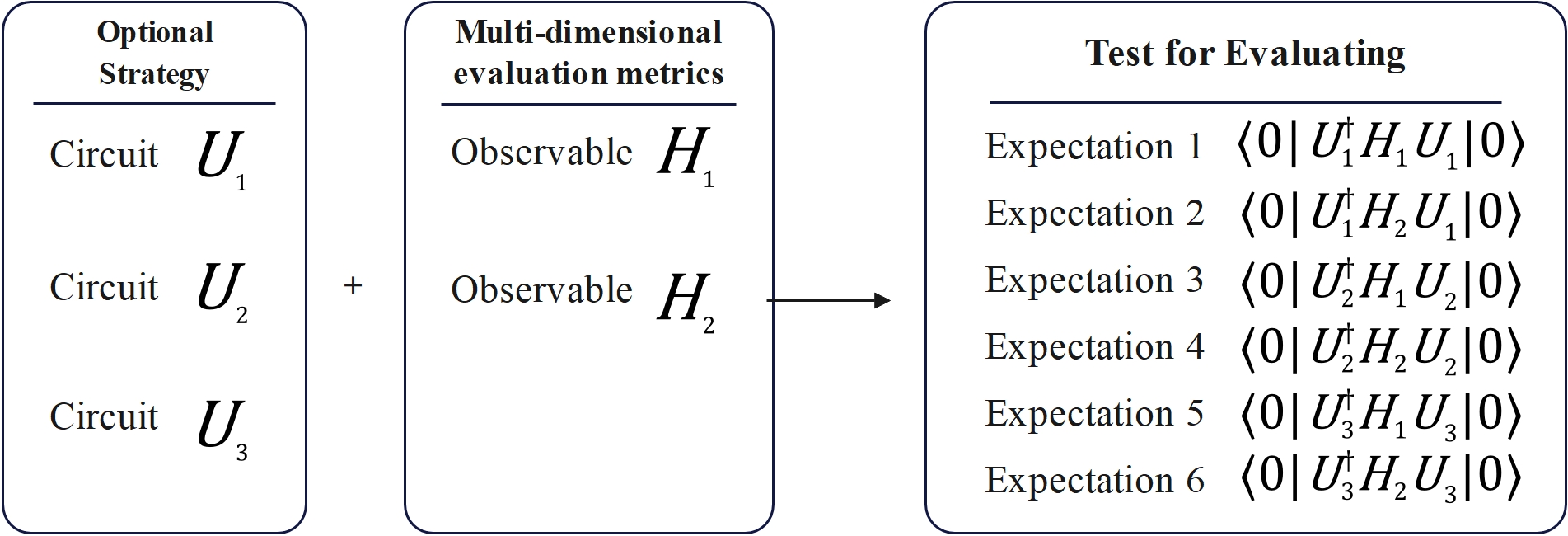
In general,

Let:

Strategy set \(\mathcal{U}=\left\{U_{1}, U_{2}, \ldots, U_{n}\right\}\) , containing n different trial circuits (strategies)
Metric set \(\mathcal{H}=\left\{H_{1}, H_{2}, \ldots, H_{m}\right\}\) , containing m different Hamiltonian observables (metric dimensions)

The evaluation process constructs the Cartesian product of these two sets:

\[ \mathcal{U} \times \mathcal{H}=\left\{\left(U_{i}, H_{j}\right) \mid U_{i} \in \mathcal{U}, H_{j} \in \mathcal{H}\right\} \]

Each element \( \left(U_{i}, H_{j}\right)\) of this product corresponds to an evaluation task: use strategy \(U_{i}\) to evaluate its performance on metric \(H_{j}\).

A Simple Example#

Step 2> Prepare trial circuits#

# python code

from pyqpanda3.core import *
prog = QProg()
prog << X(0)<<CNOT(0,1)
prog2 = QProg()
prog2 << Y(1)<<CZ(1,0)
prog3 = QProg()
prog3 << Z(0)<<SWAP(0,1)

Step 3> Prepare Hamiltonian observables#

# python code
# Continue from the previous example on this page
from pyqpanda3.hamiltonian import Hamiltonian
ham = Hamiltonian([('XZ', [0, 1], 3.14),('XZ', [0, 1], 1.14), ('ZY', [0, 1], 5.14)])
ham2 = Hamiltonian([('XZ', [0, 1], 1)])

Step 4> Use ProgramSet to manage trial circuit list and Hamiltonian observable list#

# python code
# Continue from the previous example on this page
from qpanda3_runtime import CircuitObservableBinding
progs = [prog,prog2,prog3]
hams = [ham,ham2]
cir_obs = CircuitObservableBinding(progs,hams)

Step 5> Add product rule to ProgramSet (for automatically generating combination relationships)#

Cartesian product combination relationship - CircuitObservableBinding.product
- Parameters
  - First parameter: list of indices of trial circuits in the trial circuit list
  - Second parameter: list of indices of Hamiltonian observables in the observable list
- Combination relationship illustration
```
The combinations of trial circuits and observables are: (0,0),(0,1),(1,0),(1,1),(2,0),(2,1)
```
- Analogy: Python’s itertools.product interface

# python code
# Continue from the previous example on this page
cir_obs.product([0,1,2],[0,1])

Step 6> Use ProgramSet to define and submit expectation estimation task#

# python code
# Continue from the previous example on this page
dev=service.device('72') # Here we use the quantum computing chip with id 72
task = service.estimate(
    cir_obs,
    dev,
)
res = task.get_result_sync()
print(f'res:{res}')

Complete Example Code#

# python code

from qpanda3_runtime import RuntimeService
from pyqpanda3.core import *
from pyqpanda3.hamiltonian import Hamiltonian
from qpanda3_runtime import CircuitObservableBinding

service = RuntimeService()
service.login('your_valid_api_key')
prog = QProg()
prog << X(0)<<CNOT(0,1)
prog2 = QProg()
prog2 << Y(1)<<CZ(1,0)
prog3 = QProg()
prog3 << Z(0)<<SWAP(0,1)
ham = Hamiltonian([('XZ', [0, 1], 3.14),('XZ', [0, 1], 1.14), ('ZY', [0, 1], 5.14)])
ham2 = Hamiltonian([('XZ', [0, 1], 1)])
progs = [prog,prog2,prog3]
hams = [ham,ham2]
cir_obs = CircuitObservableBinding(progs,hams)
cir_obs.product([0,1,2],[0,1])
dev=service.device('72') # Here we use the quantum computing chip with id 72
task = service.estimate(
    cir_obs,
    dev,
)
res = task.get_result_sync()
print(f'res:{res}')

More Flexible Usage#

One-to-One - Zip Rule#

Parameters
- First parameter: list of indices of trial circuits in the trial circuit list
- Second parameter: list of indices of Hamiltonian observables in the observable list
Analogy: Python’s zip interface
The automatically generated combinations of trial circuits and observables in the code below are (0,1),(2,0)

Note that the zip rule cannot obviously demonstrate performance like the product rule, but can improve the flexibility of program design

# python code

from qpanda3_runtime import RuntimeService
from pyqpanda3.core import *
from pyqpanda3.hamiltonian import Hamiltonian
from qpanda3_runtime import CircuitObservableBinding

service = RuntimeService()
service.login('your_valid_api_key')
prog = QProg()
prog << X(0)<<CNOT(0,1)
prog2 = QProg()
prog2 << Y(1)<<CZ(1,0)
prog3 = QProg()
prog3 << Z(0)<<SWAP(0,1)
ham = Hamiltonian([('XZ', [0, 1], 3.14),('XZ', [0, 1], 1.14), ('ZY', [0, 1], 5.14)])
ham2 = Hamiltonian([('XZ', [0, 1], 1)])
progs = [prog,prog2,prog3]
hams = [ham,ham2]
cir_obs = CircuitObservableBinding(progs,hams)
cir_obs.zip([0,2],[1,0])
dev=service.device('72') # Here we use the quantum computing chip with id 20
task = service.estimate(
    cir_obs,
    dev,
)
res = task.get_result_sync()
print(f'res:{res}')

Freely Add Combination Rules#

The automatically generated combinations of trial circuits and observables in the code below are (0,0),(0,1),(1,0),(1,1),(2,0),(2,1),(0,1),(2,0), where (0,0),(0,1),(1,0),(1,1),(2,0),(2,1) are generated by the product rule, and (0,1),(2,0) are generated by the zip rule

Note that the code below is only for functional demonstration. In actual application, it should be adjusted according to needs

# python code

from qpanda3_runtime import RuntimeService
from pyqpanda3.core import *
from pyqpanda3.hamiltonian import Hamiltonian
from qpanda3_runtime import CircuitObservableBinding

service = RuntimeService()
service.login('your_valid_api_key')
prog = QProg()
prog << X(0)<<CNOT(0,1)
prog2 = QProg()
prog2 << Y(1)<<CZ(1,0)
prog3 = QProg()
prog3 << Z(0)<<SWAP(0,1)
ham = Hamiltonian([('XZ', [0, 1], 3.14),('XZ', [0, 1], 1.14), ('ZY', [0, 1], 5.14)])
ham2 = Hamiltonian([('XZ', [0, 1], 1)])
progs = [prog,prog2,prog3]
hams = [ham,ham2]
cir_obs = CircuitObservableBinding(progs,hams)
cir_obs.product([0,1,2],[0,1])
cir_obs.zip([0,2],[1,0])
dev=service.device('72') # Here we use the quantum computing chip with id 72
task = service.estimate(
    cir_obs,
    dev,
)
res = task.get_result_sync()
print(f'res:{res}')