上一章: 量子线路与量子程序
下一章: 量子中间编译
简介
量子态编码是一个将经典信息转化为量子态的过程。在使用量子算法解决经典问题的过程中,量子态编码是非常重要的一步。比如在使用HHL算法解如下线性方程组时
$$\begin{aligned} \begin{aligned} A=\left(\begin{array}{cc} 1 & -1 / 3 \ -1 / 3 & 1 \end{array}\right), \vec{x}=\left(\begin{array}{l} x_{1} \ x_{2} \end{array}\right), \vec{b}=\left(\begin{array}{l} 1 \ 0 \end{array}\right) \end{aligned} \end{aligned}$$
需要将向量 b 编码至线路中。而大多数量子态编码都是以 \(\left|0\right\rangle\) 为基态进行制备,而制备后的经典信息则可以表现在量子线路的各个参数中。
本教程中我们将讨论四种量子编码的方式,包括基态编码、角度编码、振幅编码、IQP 编码。在 pyqpanda3 中,我们内置了这四类量子编码方式至 Encode 类中。
Encode 类提供了多种量子态编码方法,用于将量子态编码为不同格式的函数,其中包括编码为二进制串的基态编码,编码至角度及相位的角度编码,以及针对稀疏数据、密集数据的多种振幅编码方式,以及近似振幅编码方法。
基态编码
基态编码[1]是将一个 \(n\) 位的二进制字符串 \(x\) 转换为一个具有 \(n\) 个量子比特的系统的量子态 \(\left|x\right\rangle=\left|\psi\right\rangle\)。其中, \(\left|\psi\right\rangle\) 为转换后的计算基态。例如,当需要对一个长度为 4 的二进制字符串 \(1001\) 编码时,得到的结果即为 \(\left|1001\right\rangle\)。使用示例如下:
Python
import numpy as np
if __name__=="__main__":
qvm = CPUQVM()
x = '1001'
qubits = range(4)
cir_encode=Encode()
cir_encode.basic_encode(qubits,x)
prog = QProg()
prog << cir_encode.get_circuit()
encode_qubits = cir_encode.get_out_qubits()
qvm.run(prog,1)
result = qvm.result().get_prob_dict(encode_qubits)
print(result)
执行结果如下所示:
{'0000': 0.0, '0001': 0.0, '0010': 0.0, '0011': 0.0, '0100': 0.0, '0101': 0.0, '0110': 0.0, '0111': 0.0, '1000': 0.0, '1001': 1.0, '1010': 0.0, '1011': 0.0, '1100': 0.0, '1101': 0.0, '1110': 0.0, '1111': 0.0}
角度编码
角度编码[1]即是利用旋转门 \(R_{x}\), \(R_{y}\), \(R_{z}\) 的旋转角度进行对经典信息的编码。
$$\begin{aligned} |\boldsymbol{x}\rangle=\bigotimes_{i=1}^{N} \cos \left(x_{i}\right)|0\rangle+\sin \left(x_{i}\right)|1\rangle \end{aligned}$$ 其中 \(\left|x\right\rangle\) 即为所需编码的经典数据向量。
下面我们以 \(R_{y}\) 门编码一组角度 \([\pi,\pi]\) 为例。
Python
import numpy as np
if __name__=="__main__":
qvm = CPUQVM()
x = [np.pi,np.pi]
qubits = range(2)
cir_encode=Encode()
cir_encode.angle_encode(qubits,x)
prog = QProg()
prog << cir_encode.get_circuit()
encode_qubits = cir_encode.get_out_qubits()
qvm.run(prog,1)
result = qvm.result().get_prob_dict(encode_qubits)
print(result)
执行结果如下所示:
{'00': 1.405799628556214e-65, '01': 3.749399456654644e-33, '10': 3.749399456654644e-33, '11': 1.0}
由于一个 qubit 不仅可以加载角度信息,还可以加载相位信息,因此,我们完全可以将一个长度为 \(N\) 的经典数据编码至 \(\lceil N \rceil\) 个量子比特上。
$$\begin{aligned} |\boldsymbol{x}\rangle=\bigotimes_{i=1}^{\lceil N / 2\rceil} \cos \left(\pi x_{2 i-1}\right)|0\rangle+e^{2 \pi i x_{2 i}} \sin \left(\pi x_{2 i-1}\right)|1\rangle \end{aligned}$$
其中,将两个数据分别编码至量子特的旋转角度 \(\cos \left(\pi x_{2 i-1}\right)|0\rangle\) 与相位信息 \(e^{2 \pi i x_{2 i}} \sin \left(\pi x_{2 i-1}\right)|1\rangle\) 中。
可以发现,在经典角度编码中将经典数据向量 \(x\) 向 \(y\) 轴旋转了 \(\pi\)。由于密集角度编码会将一半信息编码至量子态的相位信息中。那么,我们可以调用 run 接口,获取系统的量子态信息。
Python
import numpy as np
if __name__=="__main__":
qvm = CPUQVM()
x = [np.pi,np.pi]
qubits = range(1)
cir_encode=Encode()
cir_encode.dense_angle_encode(qubits,x)
prog = QProg()
prog << cir_encode.get_circuit()
encode_qubits = cir_encode.get_out_qubits()
qvm.run(prog,1)
result = qvm.result().get_prob_dict(encode_qubits)
print(result)
执行结果如下所示:
{'0': 3.749399456654644e-33, '1': 1.0}
振幅编码
振幅编码即是将一个长度为 \(N\) 的数据向量 \(x\) 编码至数量为 \(\lceil log_{2}N \rceil\) 的量子比特的振幅上,具体公式如下:
$$\begin{aligned} \left|\psi\right\rangle=x_{0}|0\rangle+\cdots+x_{N-1}|N-1\rangle \end{aligned}$$
然而,可以发现由于处于纯态或混合态的量子系统的迹是为1的,所以我们需要将数据进行归一化处理,因此在接口入参时会进行校验。同时,一个编码算法需要考虑的通常有三点,分别为编码线路的深度,宽度(qubit 数量),以及 CNOT 门的数量。因此,对应以上三点,在 pyqpanda3 中也提供了不同的编码方法。同时根据数据形式的不同也可分为密集数据编码和稀疏数据编码。
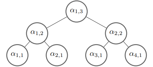
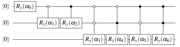
Top-down[2] 的编码方式,顾名思义,即是将数据向量先进行处理,得到对应的角度树,并从角度树的根节点开始,依次向下进行编码,如下图所示:
这种编码方式具有 \(O(\lceil log_{2} N \rceil)\) 的线路宽度,以及 \(O(n)\) 的线路深度。
Python
import numpy as np
if __name__=="__main__":
qvm = CPUQVM()
data = [0,1/np.sqrt(3),0,0,0,1/np.sqrt(3),1/np.sqrt(3),0]
data = np.asarray(data)
qubits = range(3)
cir_encode=Encode()
cir_encode.amplitude_encode(qubits,data)
prog = QProg()
prog << cir_encode.get_circuit()
print(prog)
encode_qubits = cir_encode.get_out_qubits()
qvm.run(prog,1)
result = qvm.result().get_prob_dict(encode_qubits)
print(result)
执行结果如下所示:
┌──────────────┐ ┌──────────────┐ ┌──────────────┐ >
q_0: |0>───────────────── ──────────────── ─── ──────────────── ─── ┤RY(0.00000000)├ ─── ┤RY(3.14159265)├ ─── ┤RY(0.00000000)├ >
┌──────────────┐ ┌──────────────┐ └───────┬──────┘ ┌─┐ └───────┬──────┘ ┌─┐ └───────┬──────┘ >
q_1: |0>───────────────── ┤RY(1.57079633)├ ─── ┤RY(0.00000000)├ ─── ────────*─────── ┤X├ ────────*─────── ┤X├ ────────*─────── >
┌──────────────┐ └───────┬──────┘ ┌─┐ └───────┬──────┘ ┌─┐ │ └─┘ │ ├─┤ │ >
q_2: |0>─┤RY(1.91063324)├ ────────*─────── ┤X├ ────────*─────── ┤X├ ────────*─────── ─── ────────*─────── ┤X├ ────────*─────── >
└──────────────┘ └─┘ └─┘ └─┘ >
c : / ═
┌──────────────┐
q_0: |0>─── ┤RY(3.14159265)├ ───
┌─┐ └───────┬──────┘ ┌─┐
q_1: |0>┤X├ ────────*─────── ┤X├
└─┘ │ ├─┤
q_2: |0>─── ────────*─────── ┤X├
└─┘
c : /
{'000': 1.2497998188848808e-33, '001': 0.33333333333333315, '010': 0.0, '011': 0.0, '100': 1.2497998188848817e-33, '101': 0.3333333333333334, '110': 0.3333333333333334, '111': 0.0}
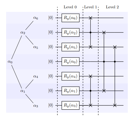
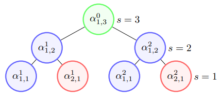
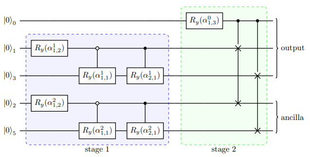
与 Top-down 编码方式相反,Bottom-top[2] 通过 \(O(n)\) 的宽度构建一个 \(O(\lceil log_{2} N \rceil)\) 深度的量子线路。其中,角度树中最左子树 ( \(\alpha_{0}\) , \(\alpha_{1}\) , \(\alpha_{3}\)) 对应的量子比特为输出比特,其余为辅助比特。构建形式如下图所示:
其中,level1 与 level2 对应的量子逻辑门为受控 SWAP 门,其作用为交换辅助比特与输出比特量子态。
Python
import numpy as np
if __name__=="__main__":
qvm = CPUQVM()
data = [0,1/np.sqrt(3),0,0,0,1/np.sqrt(3),1/np.sqrt(3),0]
data = np.asarray(data)
qubits = range(7)
cir_encode=Encode()
cir_encode.dc_amplitude_encode(qubits,data)
prog = QProg()
prog << cir_encode.get_circuit()
print(prog)
encode_qubits = cir_encode.get_out_qubits()
qvm.run(prog,1)
result = qvm.result().get_prob_dict(encode_qubits)
print(result)
执行结果如下所示:
┌──────────────┐
q_0: |0>─┤RY(1.91063324)├ ──── *─ *─
├──────────────┤ │ │
q_1: |0>─┤RY(0.00000000)├ ──*─ X─ ┼─
├──────────────┤ │ │ │
q_2: |0>─┤RY(1.57079633)├ *─┼─ X─ ┼─
├──────────────┤ │ │ │
q_3: |0>─┤RY(3.14159265)├ ┼─X─ ── X─
├──────────────┤ │ │ │
q_4: |0>─┤RY(0.00000000)├ ┼─X─ ── ┼─
├──────────────┤ │ │
q_5: |0>─┤RY(3.14159265)├ X─── ── X─
├──────────────┤ │
q_6: |0>─┤RY(0.00000000)├ X─── ── ──
└──────────────┘
c : / ═
{'000': 1.2497998188848807e-33, '001': 0.33333333333333315, '010': 0.0, '011': 0.0, '100': 1.2497998188848817e-33, '101': 0.3333333333333334, '110': 0.3333333333333334, '111': 0.0}
双向振幅编码[2]则是综合了 Top-down 和 Bottom-top 两种编码方式,即可通过参数 \(split\) 控制决定其线路深度与宽度。其线路宽度为 \(O_{w}\left(2^{split}+\log _{2}^{2}(N)-split^{2}\right)\),线路深度为 \(O_{d}\left((split+1) \frac{N}{2^{split}}\right)\),而在我们 pyqpanda 中的接口默认为 \(n/2\)。从 \(O_{w}\) 和 \(O_{d}\) 的公式可以看出当 split 为 1 时,则为 Bottom-top 振幅编码,当 spilt 为 n 时则为 Top-down 振幅编码。
Python
import numpy as np
if __name__=="__main__":
qvm = CPUQVM()
data = [0,1/np.sqrt(3),0,0,0,1/np.sqrt(3),1/np.sqrt(3),0]
data = np.asarray(data)
qubits = range(5)
cir_encode=Encode()
cir_encode.bid_amplitude_encode(qubits,data)
prog = QProg()
prog << cir_encode.get_circuit()
print(prog)
encode_qubits = cir_encode.get_out_qubits()
qvm.run(prog,1)
result = qvm.result().get_prob_dict(encode_qubits)
print(result)
执行结果如下所示:
┌──────────────┐
q_0: |0>─┤RY(1.91063324)├ ──────────────── ─── ──────────────── ─── *─ *─
├──────────────┤ ┌─┐ ┌─┐ │ │
q_1: |0>─┤RY(0.00000000)├ ────────*─────── ┤X├ ────────*─────── ┤X├ X─ ┼─
└──────────────┘ ┌───────┴──────┐ └─┘ ┌───────┴──────┐ └─┘ │ │
q_2: |0>───────────────── ┤RY(0.00000000)├ ─── ┤RY(3.14159265)├ ─── ┼─ X─
┌──────────────┐ └──────────────┘ ┌─┐ └──────────────┘ ┌─┐ │ │
q_3: |0>─┤RY(1.57079633)├ ────────*─────── ┤X├ ────────*─────── ┤X├ X─ ┼─
└──────────────┘ ┌───────┴──────┐ └─┘ ┌───────┴──────┐ └─┘ │
q_4: |0>───────────────── ┤RY(0.00000000)├ ─── ┤RY(3.14159265)├ ─── ── X─
└──────────────┘ └──────────────┘
c : / ═
{'000': 1.2497998188848807e-33, '001': 0.33333333333333315, '010': 0.0, '011': 0.0, '100': 1.2497998188848813e-33, '101': 0.3333333333333334, '110': 0.3333333333333334, '111': 0.0}
如 Top-down 振幅编码所示,使用 \(\lceil log_{2} N \rceil\) 个量子比特编码长度为: \(N\) 的经典数据大约需要 \(2^{2n}\) 个受控旋转门,这极大的降低了量子线路的保真度,然而基于schmidt分解振幅编码[3]可以有效降低线路中的受控旋转门数量。首先,一个纯态 \(|\psi\rangle\) 可以被表示为如下形式:
$$\begin{aligned} |\psi\rangle=\sum_{i=1}^{k} \lambda_{i}\left|\alpha_{i}\right\rangle \otimes\left|\beta_{i}\right\rangle \end{aligned}$$
进一步,可以表示为:
$$\begin{aligned} |\psi\rangle=\sum_{i=1}^{m} \sum_{j=1}^{n} C_{i j}\left|e_{i}\right\rangle \otimes\left|f_{j}\right\rangle \end{aligned}$$
其中, \(\left|e_{i}\right\rangle \in \mathbb{C}^{m}, \left|f_{j}\right\rangle \in \mathbb{C}^{n}\)。而 \(C\) 可以进行奇异值分解(svd) \(C=U \Sigma V^{\dagger}\),通过以上公式,我们可以得出 \(\sigma_{i i}=\lambda_{i}\), \(\left|\alpha_{i}\right\rangle=U\left|e_{i}\right\rangle\), \(\left|\beta_{i}\right\rangle=V^{\dagger}\left|f_{i}\right\rangle\),其中, \(\sigma_{i i}\) 则是 \(C\) 的奇异值。线路图构建如下:
Python
import numpy as np
if __name__=="__main__":
qvm = CPUQVM()
data = [0,1/np.sqrt(3),0,0,0,1/np.sqrt(3),1/np.sqrt(3),0]
data = np.asarray(data)
qubits = range(3)
cir_encode=Encode()
cir_encode.schmidt_encode(qubits,data)
prog = QProg()
prog << cir_encode.get_circuit()
print(prog)
encode_qubits = cir_encode.get_out_qubits()
qvm.run(prog,1)
result = qvm.result().get_prob_dict(encode_qubits)
print(result)
┌────┐ ┌───────────────────────────────────────────────────┐ >
q_0: |0>─────────────────────────────────────────────────────── ┤CNOT├ ┤U4(0.00000000, 1.57079633, 2.12437069, -3.14159265)├ >
┌────────────────────────────────────────────────────┐ └──┬─┘ └───────────────────────────────────────────────────┘ >
q_1: |0>─┤U4(-0.00000000, 3.14159265, 0.00000000, -3.14159265)├ ───┼── ───────────────────────────────────────────────────── >
├──────────────┬─────────────────────────────────────┘ │ ┌───────────────────────────────────────────────────┐ >
q_2: |0>─┤RY(0.72972766)├────────────────────────────────────── ───*── ┤U4(1.57079633, 0.00000000, 2.03444394, -3.14159265)├ >
└──────────────┘ └───────────────────────────────────────────────────┘ >
c : / ═
┌────────────────────────────────────────────────────┐ ┌───────────────────────────────────────────────────┐
q_0: |0>──*─ ┤U4(-0.00000000, -0.00000000, 2.12437069, 4.71238898)├ ──*─ ┤U4(-0.00000000, 0.46364761, 0.00000000, 1.10714872)├─
┌─┴┐ ├──────────────────────────────────────────────────┬─┘ ┌─┴┐ ├───────────────────────────────────────────────────┴┐
q_1: |0>┤CZ├ ┤U4(0.00000000, 0.00000000, 1.57079633, 1.57079633)├── ┤CZ├ ┤U4(0.78539816, -1.57079633, 1.57079633, -6.28318531)├
└──┘ └──────────────────────────────────────────────────┘ └──┘ └────────────────────────────────────────────────────┘
q_2: |0>──── ────────────────────────────────────────────────────── ──── ──────────────────────────────────────────────────────
c : /
{'000': 3.51862174721677e-32, '001': 0.33333333333333315, '010': 4.8452179519763874e-32, '011': 3.505620428081208e-33, '100': 1.025086436597375e-31, '101': 0.3333333333333338, '110': 0.3333333333333329, '111': 2.723201269651864e-32}
MPS近似编码[4]是一种利用矩阵乘积态的低秩表达近似分布制备算法,可以通过一种较少的 CNOT 的门完成对分布的表达,并且这种表达是一种近邻接形式,因此可以直接作用于芯片,且双门个数的减少,也有利于增加分布制备的成功率,量子线路图如下所示。
可以发现该函数支持多种类型数据制备(double,complex),其中 layers 指的是使用矩阵乘积态近似的层数,sweeps 是指通过环境张量优化的迭代次数。环境张量的数学表达如下:
$$\begin{aligned} \hat{\mathcal{F}}_m=\operatorname{Tr}_{\bar{U}_m}\left[\prod_{i=M}^{m+1} U_i\left|\psi_{\chi_{\max }}\right\rangle\left\langle 0^{\otimes N}\right| \prod_{j=1}^{m-1} U_j^{\dagger}\right] \end{aligned}$$
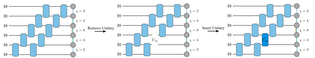
其中, \(\operatorname{Tr}_{\bar{U}_m}\) 指的是不与 \(U_m\) 相互作用的量子比特索引上的偏迹,环境张量 \(\hat{\mathcal{F}}_m\) 则被表示为一个 \(4×4\) 的矩阵,在实际中可以通过从量子线路中移除 \(U_m\) 并收缩剩余的张量来计算(见下图),并同时始终保持 MPS 结构。最后,为了适配芯片的拓扑结构,该制备算法的 \(chi\) 均为 2。
下面,我们以 W-state 作为示例,展示 MPS 近似编码的神奇,即在无论多少比特的 W-state,均可在一层解纠缠下完成准确编码。因此,针对纠缠度较低的数据,如正太分布数据,可在一个较低深度下近似表达。
Python
import numpy as np
if __name__=="__main__":
qvm = CPUQVM()
data = [0,1/np.sqrt(3),0,0,0,1/np.sqrt(3),1/np.sqrt(3),0]
data = np.asarray(data)
qubits = range(3)
cir_encode=Encode()
cir_encode.approx_mps_encode(qubits,data)
prog = QProg()
prog << cir_encode.get_circuit()
print(prog)
encode_qubits = cir_encode.get_out_qubits()
qvm.run(prog,1)
result = qvm.result().get_prob_dict(encode_qubits)
print(result)
┌───────────────────────────────────────────────────┐ ┌───────────────────────────────────────────────────┐ >
q_0: |0>─┤U4(-0.00000000, 1.57079633, 0.14422034, 3.14159265)├─ ──*─ ┤U4(0.00000000, -3.14159265, 3.02600465, 1.57079633)├─ >
├──────────────────────────────────────────────────┬┘ ┌─┴┐ ├───────────────────────────────────────────────────┴┐ >
q_1: |0>─┤U4(0.00000000, 1.57079633, 2.52929625, 0.00000000)├── ┤CZ├ ┤U4(-0.00000000, 3.14159265, 0.93069872, -1.57079633)├ >
├──────────────────────────────────────────────────┴─┐ └──┘ └────────────────────────────────────────────────────┘ >
q_2: |0>─┤U4(0.00000000, -1.57079633, 2.62654637, -3.14159265)├ ──── ────────────────────────────────────────────────────── >
└────────────────────────────────────────────────────┘ >
c : / ═
┌──────────────────────────────────────────────────┐ ┌───────────────────────────────────────────────────┐ >
q_0: |0>──*─ ┤U4(0.00000000, 0.00000000, 2.74728685, 0.00000000)├── ┤U4(-0.00000000, 2.44026625, 1.57079633, 1.57079633)├ >
┌─┴┐ ├──────────────────────────────────────────────────┴─┐ ├───────────────────────────────────────────────────┤ >
q_1: |0>┤CZ├ ┤U4(-0.00000000, 3.14159265, 1.60338538, -3.14159265)├ ┤U4(0.00000000, 4.71238898, 1.16262513, -0.00000000)├ >
└──┘ └────────────────────────────────────────────────────┘ └───────────────────────────────────────────────────┘ >
q_2: |0>──── ────────────────────────────────────────────────────── ───────────────────────────────────────────────────── >
>
c : /
>
q_0: |0>──── ───────────────────────────────────────────────────── ──── ────────────────────────────────────────────────────── >
┌───────────────────────────────────────────────────┐ ┌───────────────────────────────────────────────────┐ >
q_1: |0>──*─ ┤U4(0.00000000, -3.14159265, 1.77399044, 1.57079633)├ ──*─ ┤U4(0.00000000, -3.14159265, 1.51402457, 3.14159265)├─ >
┌─┴┐ ├───────────────────────────────────────────────────┤ ┌─┴┐ ├───────────────────────────────────────────────────┴┐ >
q_2: |0>┤CZ├ ┤U4(0.00000000, 3.14159265, 1.39084874, -1.57079633)├ ┤CZ├ ┤U4(-0.00000000, -3.14159265, 1.24134660, 3.14159265)├ >
└──┘ └───────────────────────────────────────────────────┘ └──┘ └────────────────────────────────────────────────────┘ >
c : /
┌───────────────────────────────────────────────────┐ >
q_0: |0>─────────────────────────────────────────────────────── ──*─ ┤U4(0.00000000, -3.14159265, 3.09540078, 1.57079633)├ >
┌─────────────────────────────────────────────────────┐ ┌─┴┐ ├───────────────────────────────────────────────────┤ >
q_1: |0>┤U4(-0.00000000, -3.32978396, 1.57079633, -1.57079633)├ ┤CZ├ ┤U4(0.00000000, 3.14159265, 0.31160284, -1.57079633)├ >
├───────────────────────────────────────────────────┬─┘ └──┘ └───────────────────────────────────────────────────┘ >
q_2: |0>┤U4(0.00000000, -0.41642121, 1.57079633, 1.57079633)├── ──── ───────────────────────────────────────────────────── >
└───────────────────────────────────────────────────┘ >
c : /
┌───────────────────────────────────────────────────┐ ┌───────────────────────────────────────────────────┐ >
q_0: |0>──*─ ┤U4(-0.00000000, 4.71238898, 1.57079633, 1.08485200)├ ┤U4(0.00000000, 1.57079633, 1.03964616, -3.14159265)├ >
┌─┴┐ ├───────────────────────────────────────────────────┤ ├───────────────────────────────────────────────────┤ >
q_1: |0>┤CZ├ ┤U4(1.57079633, -1.57079633, 1.57079633, 1.76216405)├ ┤U4(0.00000000, 0.00000000, 1.85661223, -0.00000000)├ >
└──┘ └───────────────────────────────────────────────────┘ └───────────────────────────────────────────────────┘ >
q_2: |0>──── ───────────────────────────────────────────────────── ───────────────────────────────────────────────────── >
>
c : /
>
q_0: |0>──── ─────────────────────────────────────────────────────── ──── ────────────────────────────────────────────────────── >
┌───────────────────────────────────────────────────┐ ┌────────────────────────────────────────────────────┐ >
q_1: |0>──*─ ┤U4(0.00000000, -1.57079633, 0.13083119, 4.71238898)├── ──*─ ┤U4(-0.00000000, 3.14159265, 0.04863628, -1.57079633)├ >
┌─┴┐ ├───────────────────────────────────────────────────┴─┐ ┌─┴┐ ├───────────────────────────────────────────────────┬┘ >
q_2: |0>┤CZ├ ┤U4(-0.00000000, -0.00000000, 1.57079633, -0.00000000)├ ┤CZ├ ┤U4(0.00000000, -1.57079633, 1.57079633, 3.14159265)├─ >
└──┘ └─────────────────────────────────────────────────────┘ └──┘ └───────────────────────────────────────────────────┘ >
c : /
>
q_0: |0>──── ────────────────────────────────────────────────────── ─────────────────────────────────────────────────────── >
┌────────────────────────────────────────────────────┐ ┌─────────────────────────────────────────────────────┐ >
q_1: |0>──*─ ┤U4(0.00000000, -0.00000000, 2.38474385, -4.71238898)├ ┤U4(-0.00000000, -0.00000000, 0.41015532, -3.14159265)├ >
┌─┴┐ ├───────────────────────────────────────────────────┬┘ ├────────────────────────────────────────────────────┬┘ >
q_2: |0>┤CZ├ ┤U4(1.57079633, -7.85398163, 1.57079633, 1.05132326)├─ ┤U4(-0.00000000, 0.00000000, 2.83411843, -3.14159265)├─ >
└──┘ └───────────────────────────────────────────────────┘ └────────────────────────────────────────────────────┘ >
c : /
┌───────────────────────────────────────────────────┐ ┌───────────────────────────────────────────────────┐ >
q_0: |0>──*─ ┤U4(0.00000000, -1.57079633, 0.23969156, 4.71238898)├── ──*─ ┤U4(0.00000000, -0.00000000, 0.05916140, 1.57079633)├ >
┌─┴┐ ├───────────────────────────────────────────────────┴─┐ ┌─┴┐ ├───────────────────────────────────────────────────┤ >
q_1: |0>┤CZ├ ┤U4(-0.00000000, -0.00000000, 1.57079633, -0.00000000)├ ┤CZ├ ┤U4(0.00000000, -1.57079633, 1.57079633, 3.14159265)├ >
└──┘ └─────────────────────────────────────────────────────┘ └──┘ └───────────────────────────────────────────────────┘ >
q_2: |0>──── ─────────────────────────────────────────────────────── ──── ───────────────────────────────────────────────────── >
>
c : /
┌───────────────────────────────────────────────────┐ >
q_0: |0>──*─ ┤U4(0.00000000, 3.14159265, 0.91540970, -3.14159265)├─ ───────────────────────────────────────────────────── >
┌─┴┐ ├───────────────────────────────────────────────────┴┐ ┌───────────────────────────────────────────────────┐ >
q_1: |0>┤CZ├ ┤U4(1.57079633, -3.14159265, 2.89220717, -1.57079633)├ ┤U4(0.00000000, 4.71238898, 1.09507112, -0.00000000)├ >
└──┘ └────────────────────────────────────────────────────┘ └───────────────────────────────────────────────────┘ >
q_2: |0>──── ────────────────────────────────────────────────────── ───────────────────────────────────────────────────── >
>
c : /
q_0: |0>──── ─────────────────────────────────────────────────────── ──── ────────────────────────────────────────────────────── ──── ──────────────────────────────────────────────────────
┌───────────────────────────────────────────────────┐ ┌────────────────────────────────────────────────────┐ ┌────────────────────────────────────────────────────┐
q_1: |0>──*─ ┤U4(0.00000000, -1.57079633, 0.24153608, 4.71238898)├── ──*─ ┤U4(-0.00000000, 3.14159265, 0.13122312, -1.57079633)├ ──*─ ┤U4(0.00000000, -3.14159265, 0.62086323, -0.00000000)├
┌─┴┐ ├───────────────────────────────────────────────────┴─┐ ┌─┴┐ ├───────────────────────────────────────────────────┬┘ ┌─┴┐ ├───────────────────────────────────────────────────┬┘
q_2: |0>┤CZ├ ┤U4(-0.00000000, -0.00000000, 1.57079633, -0.00000000)├ ┤CZ├ ┤U4(0.00000000, -1.57079633, 1.57079633, 3.14159265)├─ ┤CZ├ ┤U4(1.57079633, -3.14159265, 1.13824884, 1.57079633)├─
└──┘ └─────────────────────────────────────────────────────┘ └──┘ └───────────────────────────────────────────────────┘ └──┘ └───────────────────────────────────────────────────┘
c : /
{'000': 1.8649098631244054e-31, '001': 0.3333333333333338, '010': 6.214926642473421e-31, '011': 3.0992622541939764e-31, '100': 7.662665571759249e-31, '101': 0.3333333333333339, '110': 0.33333333333333254, '111': 1.1994732202454884e-30}
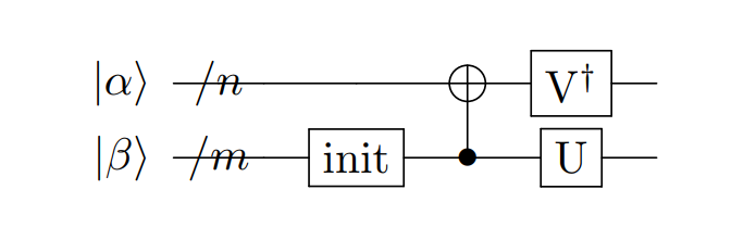
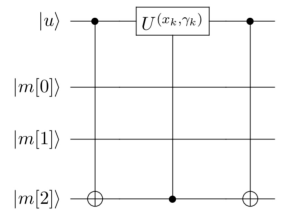
双稀疏量子态编码[5]通过利用 \(n\) 个辅助比特辅助构建线路。我们以编码 \(|001\rangle\) 为例,如下图所示:
其中, \(|\mu\rangle\) 为辅助寄存器用以作用旋转门,并受输出寄存器 \(|m\rangle\) 控制,而当所需编码的字符下标的 1 的个数较多时,则需要作用多控门,而为了减少消除线路中多控门的数量,我们通过增加一部分辅助寄存器,并利用 Toffoli 门进行分解,其原理如下图所示:
Python
import numpy as np
if __name__=="__main__":
qvm = CPUQVM()
data = [0,1/np.sqrt(3),0,0,0,1/np.sqrt(3),1/np.sqrt(3),0]
data = np.asarray(data)
qubits = range(6)
cir_encode=Encode()
cir_encode.ds_quantum_state_preparation(qubits,data)
prog = QProg()
prog << cir_encode.get_circuit()
print(prog)
encode_qubits = cir_encode.get_out_qubits()
qvm.run(prog,1)
result = qvm.result().get_prob_dict(encode_qubits)
print(result)
┌─┐ ┌───────────────────────────────────────┐ ┌───────────────────────────────────────┐ >
q_0: |0>─┤X├ ───*── ┤U3(-1.23095942, 0.00000000, 0.00000000)├ ───*── ───*── ───*── ─── ┤U3(-1.57079633, 0.00000000, 0.00000000)├ >
└─┘ │ └───────────────────┬───────────────────┘ │ │ │ ┌─┐ └───────────────────┬───────────────────┘ >
q_2: |0>──── ───┼── ────────────────────┼──────────────────── ───┼── ───┼── ───┼── ┤X├ ────────────────────*──────────────────── >
┌──┴─┐ │ ┌──┴─┐ ┌──┴─┐ │ └┬┘ >
q_3: |0>──── ┤CNOT├ ────────────────────*──────────────────── ┤CNOT├ ┤CNOT├ ───┼── ─*─ ───────────────────────────────────────── >
└────┘ └────┘ └────┘ │ │ >
q_4: |0>──── ────── ───────────────────────────────────────── ────── ────── ───┼── ─┼─ ───────────────────────────────────────── >
┌──┴─┐ │ >
q_5: |0>──── ────── ───────────────────────────────────────── ────── ────── ┤CNOT├ ─*─ ───────────────────────────────────────── >
└────┘ >
c : / ═
┌───────────────────────────────────────┐
q_0: |0>─── ───*── ───*── ───*── ───*── ─── ┤U3(-3.14159265, 0.00000000, 0.00000000)├ ───
┌─┐ │ │ │ │ ┌─┐ └───────────────────┬───────────────────┘ ┌─┐
q_2: |0>┤X├ ───┼── ───┼── ───┼── ───┼── ┤X├ ────────────────────*──────────────────── ┤X├
└┬┘ ┌──┴─┐ │ │ │ └┬┘ └┬┘
q_3: |0>─*─ ┤CNOT├ ───┼── ───┼── ───┼── ─┼─ ───────────────────────────────────────── ─┼─
│ └────┘ │ ┌──┴─┐ │ │ │
q_4: |0>─┼─ ────── ───┼── ┤CNOT├ ───┼── ─*─ ───────────────────────────────────────── ─*─
│ ┌──┴─┐ └────┘ ┌──┴─┐ │ │
q_5: |0>─*─ ────── ┤CNOT├ ────── ┤CNOT├ ─*─ ───────────────────────────────────────── ─*─
└────┘ └────┘
c : /
{'000': 0.0, '001': 0.3333333333333334, '010': 0.0, '011': 0.0, '100': 0.0, '101': 0.3333333333333333, '110': 0.33333333333333315, '111': 0.0}
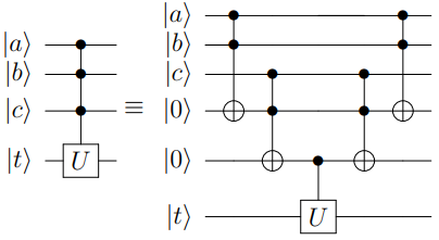
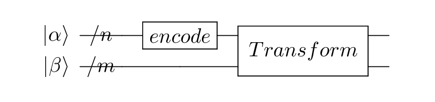
sparse_isometry 编码[6]不同于双稀疏量子态编码需要辅助比特去构建线路。sparse_isometry 编码首先通过将长度为 \(N\) 稀疏数据向量中的非 0 元素 \(x\) 统一编码至前 \(\lceil log_2len(x) \rceil\) 个量子比特上,后通过受控X门对其进行受控转化。其线路构建如下图所示:
其中, \(n+m=\lceil log_2N \rceil\) \(|\alpha\rangle\) 为 \(\lceil log_2len(x) \rceil\) 个非 0 元素的编码 encode 模块,而 \(|\beta\rangle\) 则为剩余 qubit。其中 transform 模块则是转化模块。
Python
import numpy as np
if __name__=="__main__":
qvm = CPUQVM()
data = [0,1/np.sqrt(3),0,0,0,1/np.sqrt(3),1/np.sqrt(3),0]
data = np.asarray(data)
qubits = range(3)
cir_encode=Encode()
cir_encode.sparse_isometry(qubits,data)
prog = QProg()
prog << cir_encode.get_circuit()
print(prog)
encode_qubits = cir_encode.get_out_qubits()
qvm.run(prog,1)
result = qvm.result().get_prob_dict(encode_qubits)
print(result)
python
┌──────────────┐ ┌──────────────┐ ┌─┐ ┌─┐ ┌─┐ ┌─┐ ┌─┐ ┌─┐
q_0: |0>───────────────── ┤RY(0.00000000)├ ─── ┤RY(1.57079633)├ ┤X├ ─*─ ┤X├ ┤X├ ┤X├ ─*─ ┤X├ ┤X├
┌──────────────┐ └───────┬──────┘ ┌─┐ └───────┬──────┘ ├─┤ │ ├─┤ └┬┘ └─┘ │ ├─┤ └┬┘
q_1: |0>─┤RY(1.23095942)├ ────────*─────── ┤X├ ────────*─────── ┤X├ ─*─ ┤X├ ─┼─ ─── ─*─ ┤X├ ─┼─
└──────────────┘ └─┘ └─┘ ┌┴┐ └─┘ │ ┌┴┐ └─┘ │
q_2: |0>───────────────── ──────────────── ─── ──────────────── ─── ┤X├ ─── ─*─ ─── ┤X├ ─── ─*─
└─┘ └─┘
c : / ═
{'000': 0.0, '001': 0.3333333333333333, '010': 0.0, '011': 0.0, '100': 0.0, '101': 0.33333333333333315, '110': 0.3333333333333334, '111': 0.0}
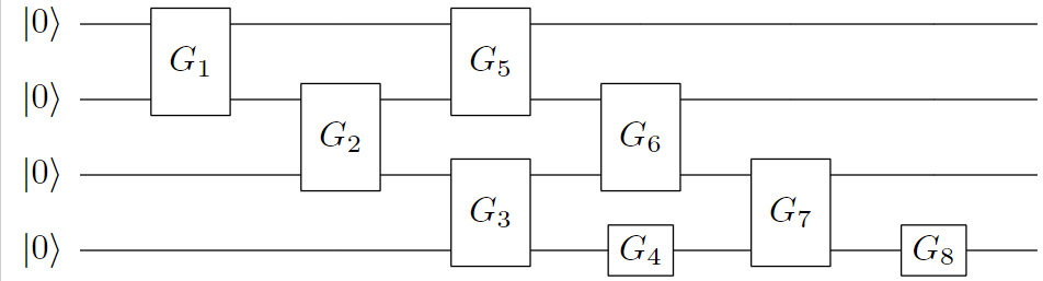
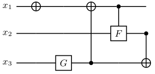
多项式稀疏量子态编码[7] 是一种稀疏数据向量中的非 0 元素个数与 qubit 个数成线性关系的稀疏数据编码方式。其线路编码深度为 \(O\left(|S|^{2} \log (|S|) n\right)\)。其中, \(|S|\) 为非 0 元素个数, \(n\) 为所需 qubit 个数,即为 \(\lceil log_2N \rceil\), \(N\) 为稀疏数据长度。下面以编码 \(|x\rangle=1/\sqrt{3}(|001\rangle+|100\rangle+|111\rangle)\) 为例,其线路图构建如下:
其中,F 门是将 \(|0\rangle\) 映射到 \(1/\sqrt{3}|0\rangle+1/\sqrt{3}|1\rangle\),而 G 门则是将 \(|0\rangle\) 映射到 \(1/\sqrt{3}|0\rangle+2/\sqrt{3}|1\rangle\)。
Python
import numpy as np
if __name__=="__main__":
qvm = CPUQVM()
data = [0,1/np.sqrt(3),0,0,0,1/np.sqrt(3),1/np.sqrt(3),0]
data = np.asarray(data)
qubits = range(3)
cir_encode=Encode()
cir_encode.efficient_sparse(qubits,data)
prog = QProg()
prog << cir_encode.get_circuit()
print(prog)
encode_qubits = cir_encode.get_out_qubits()
qvm.run(prog,1)
result = qvm.result().get_prob_dict(encode_qubits)
print(result)
┌─┐ ┌────┐ ┌────┐
q_0: |0>─┤X├ ──────────────────────────────────────── ┤CNOT├ ────── ──────────────────────────────────────── ┤CNOT├ ────── ───
└─┘ └──┬─┘ ┌────┐ └──┬─┘ ┌────┐
q_1: |0>──── ──────────────────────────────────────── ───┼── ┤CNOT├ ────────────────────*─────────────────── ───┼── ┤CNOT├ ───
┌─┐ ┌──────────────────────────────────────┐ │ └──┬─┘ ┌───────────────────┴──────────────────┐ │ └──┬─┘ ┌─┐
q_2: |0>─┤X├ ┤U3(1.23095942, 0.00000000, 0.00000000)├ ───*── ───*── ┤U3(1.57079633, 0.00000000, 0.00000000)├ ───*── ───*── ┤X├
└─┘ └──────────────────────────────────────┘ └──────────────────────────────────────┘ └─┘
c : / ═
{'000': 0.0, '001': 0.33333333333333315, '010': 0.0, '011': 0.0, '100': 0.0, '101': 0.3333333333333334, '110': 0.3333333333333333, '111': 0.0}
IQP编码
IQP编码[8] 是一种应用于量子机器学习的编码方法。将一个经典数据 x 编码到
$$\begin{aligned} |\mathbf{x}\rangle=\left(\mathrm{U}_{\mathrm{Z}}(\mathbf{x}) \mathrm{H}^{\otimes n}\right)^{\boldsymbol{r}}\left|0^{n}\right\rangle \end{aligned}$$
其中, \(r\) 表示量子线路的深度,也就是 \(\mathrm{U}_{\mathrm{Z}}(\mathbf{x}) \mathrm{H}^{\otimes n}\) 重复的次数。 \(\mathrm{H}^{\otimes n}\) 是一层作用在所有量子比特上的 Hadamard 门。其中, \(\mathrm{U}_\mathrm{Z}\) 为
$$\begin{aligned} \mathrm{U}_\mathrm{Z}(\mathbf{x})=\prod_{[i, j] \in S} R_{Z_{i} Z_{j}}\left(x_{i} x_{j}\right) \bigotimes_{k=1}^{n} R_{z}\left(x_{k}\right) \end{aligned}$$
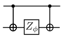
这里的 \(S\) 是一个集合,对于这个集合中的每一对量子比特,我们都需要对它们作用 \(R_{ZZ}\) 门。 \(R_{ZZ}\) 门的构建形式如下:
.align-center
下面我们以编码 \(data=[-1.3, 1.8, 2.6, -0.15]\) 为例介绍:
Python
import numpy as np
if __name__=="__main__":
qvm = CPUQVM()
data = [-1.3, 1.8, 2.6, -0.15]
data = np.asarray(data)
qubits = range(4)
cir_encode=Encode()
cir_encode.iqp_encode(qubits,data)
prog = QProg()
prog << cir_encode.get_circuit()
print(prog)
encode_qubits = cir_encode.get_out_qubits()
qvm.run(prog,1)
result = qvm.result().get_prob_dict(encode_qubits)
print(result)
┌─┐ ┌───────────────┐
q_0: |0>─┤H├ ┤RZ(-1.30000000)├ ───*── ───────────────── ───*── ────── ──────────────── ────── ────── ───────────────── ──────
├─┤ ├──────────────┬┘ ┌──┴─┐ ┌───────────────┐ ┌──┴─┐
q_1: |0>─┤H├ ┤RZ(1.80000000)├─ ┤CNOT├ ┤RZ(-2.34000000)├ ┤CNOT├ ───*── ──────────────── ───*── ────── ───────────────── ──────
├─┤ ├──────────────┤ └────┘ └───────────────┘ └────┘ ┌──┴─┐ ┌──────────────┐ ┌──┴─┐
q_2: |0>─┤H├ ┤RZ(2.60000000)├─ ────── ───────────────── ────── ┤CNOT├ ┤RZ(4.68000000)├ ┤CNOT├ ───*── ───────────────── ───*──
├─┤ ├──────────────┴┐ └────┘ └──────────────┘ └────┘ ┌──┴─┐ ┌───────────────┐ ┌──┴─┐
q_3: |0>─┤H├ ┤RZ(-0.15000000)├ ────── ───────────────── ────── ────── ──────────────── ────── ┤CNOT├ ┤RZ(-0.39000000)├ ┤CNOT├
└─┘ └───────────────┘ └────┘ └───────────────┘ └────┘
c : / ═
{'0000': 0.06250000000000001, '0001': 0.06250000000000001, '0010': 0.06250000000000004, '0011': 0.06249999999999999, '0100': 0.06250000000000001, '0101': 0.06250000000000003, '0110': 0.06250000000000001, '0111': 0.06250000000000001, '1000': 0.06250000000000001, '1001': 0.0625, '1010': 0.06250000000000003, '1011': 0.0625, '1100': 0.0625, '1101': 0.06250000000000004, '1110': 0.06250000000000001, '1111': 0.06250000000000003}
参考文献
[1] Schuld, Maria. "Quantum machine learning models are kernel methods."[J] arXiv:2101.11020 (2021).
[2] Araujo I F, Park D K, Ludermir T B, et al. "Configurable sublinear circuits for quantum state preparation."[J]. arXiv preprint arXiv:2108.10182, 2021.
[3] Ghosh K. "Encoding classical data into a quantum computer"[J]. arXiv preprint arXiv:2107.09155, 2021.
[4] Rudolph M S, Chen J, Miller J, et al. Decomposition of matrix product states into shallow quantum circuits[J]. arXiv preprint arXiv:2209.00595, 2022.
[5] de Veras T M L, da Silva L D, da Silva A J. "Double sparse quantum state preparation"[J]. arXiv preprint arXiv:2108.13527, 2021.
[6] Malvetti E, Iten R, Colbeck R. "Quantum circuits for sparse isometries"[J]. Quantum, 2021, 5: 412.
[7] N. Gleinig and T. Hoefler, "An Efficient Algorithm for Sparse Quantum State Preparation," 2021 58th ACM/IEEE Design Automation Conference (DAC), 2021, pp. 433-438, doi: 10.1109/DAC18074.2021.9586240.
[8] Havlíček, Vojtěch, et al. "Supervised learning with quantum-enhanced feature spaces." Nature 567.7747 (2019): 209-212.